Transcription
RoboticsChapter 25Chapter 251
OutlineRobots, Effectors, and SensorsLocalization and MappingMotion PlanningMotor ControlChapter 252
Mobile RobotsChapter 253
ManipulatorsPRRRRRConfiguration of robot specified by 6 numbers 6 degrees of freedom (DOF)6 is the minimum number required to position end-effector arbitrarily.For dynamical systems, add velocity for each DOF.Chapter 254
Non-holonomic robotsθ(x, y)A car has more DOF (3) than controls (2), so is non-holonomic;cannot generally transition between two infinitesimally close configurationsChapter 255
SensorsRange finders: sonar (land, underwater), laser range finder, radar (aircraft),tactile sensors, GPSImaging sensors: cameras (visual, infrared)Proprioceptive sensors: shaft decoders (joints, wheels), inertial sensors,force sensors, torque sensorsChapter 256
Localization—Where Am I?Compute current location and orientation (pose) given observations:At 2At 1AtXt 1XtXt 1Zt 1ZtZt 1Chapter 257
Localization contd.ω t txi, yiθt 1h(xt)vt tZ1Z2Z3Z4xt 1θtxtAssume Gaussian noise in motion prediction, sensor range measurementsChapter 258
Localization contd.Can use particle filtering to produce approximate position estimateRobot positionRobot positionRobot positionChapter 259
Localization contd.Can also use extended Kalman filter for simple cases:robotlandmarkAssumes that landmarks are identifiable—otherwise, posterior is multimodalChapter 2510
MappingLocalization: given map and observed landmarks, update pose distributionMapping: given pose and observed landmarks, update map distributionSLAM: given observed landmarks, update pose and map distributionProbabilistic formulation of SLAM:add landmark locations L1, . . . , Lk to the state vector,proceed as for localizationChapter 2511
Mapping contd.Chapter 2512
3D Mapping exampleChapter 2513
Motion PlanningIdea: plan in configuration space defined by the robot’s DOFsconf-2conf-1conf-3conf-3conf-2conf-1w elbw shouSolution is a point trajectory in free C-spaceChapter 2514
Configuration space planningBasic problem: d states! Convert to finite state space.Cell decomposition:divide up space into simple cells,each of which can be traversed “easily” (e.g., convex)Skeletonization:identify finite number of easily connected points/linesthat form a graph such that any two points are connectedby a path on the graphChapter 2515
Cell decomposition examplegoalstartgoalstartProblem: may be no path in pure freespace cellsSolution: recursive decomposition of mixed (free obstacle) cellsChapter 2516
Skeletonization: Voronoi diagramVoronoi diagram: locus of points equidistant from obstaclesProblem: doesn’t scale well to higher dimensionsChapter 2517
Skeletonization: Probabilistic RoadmapA probabilistic roadmap is generated by generating random points in C-spaceand keeping those in freespace; create graph by joining pairs by straight linesProblem: need to generate enough points to ensure that every start/goalpair is connected through the graphChapter 2518
Motor controlCan view the motor control problem as a search problemin the dynamic rather than kinematic state space:– state space defined by x1, x2, . . . , x 1, x 2, . . .– continuous, high-dimensional (Sarcos humanoid: 162 dimensions)Deterministic control: many problems are exactly solvableesp. if linear, low-dimensional, exactly known, observableSimple regulatory control laws are effective for specified motionsStochastic optimal control: very few problems exactly solvable approximate/adaptive methodsChapter 2519
Biological motor controlMotor control systems are characterized by massive redundancyInfinitely many trajectories achieve any given taskE.g., 3-link arm moving in plane throwing at a targetsimple 12-parameter controller, one degree of freedom at target11-dimensional continuous space of optimal controllersIdea: if the arm is noisy, only “one” optimal policy minimizes error at targetI.e., noise-tolerance might explain actual motor behaviourHarris & Wolpert (Nature, 1998): signal-dependent noiseexplains eye saccade velocity profile perfectlyChapter 2520
SetupSuppose a controller has “intended” control parameters θ0which are corrupted by noise, giving θ drawn from Pθ0Output (e.g., distance from target) y F (θ);yChapter 2521
Simple learning algorithm: Stochastic gradientMinimize Eθ [y 2] by gradient descent:2Z θ0 Eθ [y ] θ0 Pθ0 (θ)F (θ)2dθZ P (θ)θ0 θ0F (θ)2Pθ0 (θ)dθ Pθ0 (θ) θ Pθ (θ) Eθ [ 0 0 y 2 ]Pθ0 (θ)Given samples (θj , yj ), j 1, . . . , N , we have1 θ0 Eˆθ [y 2] N θ0 Pθ0 (θj ) 2yjj 1 Pθ0 (θj )NXFor Gaussian noise with covariance Σ, i.e., Pθ0 (θ) N (θ0, Σ), we obtain1ˆ2 θ0 Eθ [y ] NNXj 1Σ 1(θj θ0)yj2Chapter 2522
What the algorithm is doingxxx x xxx x x xxx xxxx x xxxx xx xxxxxxxxx xxxx xx x xx xxChapter 2523
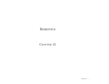
Results for 2–D controller10Velocity v9876540.20.40.60.8Angle phi11.2Chapter 2524
Results for 2–D controller4.614.64.59Velocity gle phi0.640.65Chapter 2525
Results for 2–D controller0.00950.0090.0085E(y ep800010000Chapter 2526
SummaryThe rubber hits the roadMobile robots and manipulatorsDegrees of freedom to define robot configurationLocalization and mapping as probabilistic inference problems(require good sensor and motion models)Motion planning in configuration spacerequires some method for finitizationChapter 2527
Robotics Chapter 25 Chapter 25 1. Outline Robots, E ectors, and Sensors Localization and Mapping Motion Planning Motor Control Chapter 25 2. Mobile Robots Chapter 25 3. Manipulators R R R P R R Con guration of robot speci ed by 6 numbers) 6 degrees of freedom (DOF) 6 is the min