WIXLIB

is taken into account with a simplified lunar position. In the full ephemerides model, the Earth gravitationalpotential, including the main harmonic terms of (2,0) (2,2) (3,0) (3,1) (4,0) and the point gravitational sourcesof the Sun, the Moon and Jupiter, and SRP have been taken into account. For the Jupiter’s, lunar, and solarposition, precise SPICE ephemerides are used. The solar radiation pressure model is a cannonball model witha one-meter diameter with a diffuse reflection coefficient of 0.5 and an area-to-mass ratio of 0.02 m2 /kg.ORBIT SELECTIONAs is apparent from the preliminary analysis, accelerations throughout the cislunar region are much morevariable than in the near-Earth domain. Such variability offers a much broader array of orbits and transferpaths throughout the region. A number of orbital families, for example, are not available under a two-bodyor conic model. Rather, some less familiar orbital families emerge with different types of characteristics tobe leveraged for new types of activities. Conversely, this variation also delivers new challenges for efforts tosupport orbital catalogs and predictions of behaviors in this regime. In an effort to explore the challenges,some orbits are selected to examine the acceleration levels as well as prediction. The sample obits for somepreliminary analysis include Distant Retrograde orbits (DROs) and Lyapunov orbits. In addition, a transferorbit is introduced as a type or orbital path through the entire cislunar region.resonant orbits are introduced as some options that will flow, over time, through the entire cislunar region.Earth-Moon Distant Retrogrades Orbits (DROs)Distant retrograde orbits, or DROs, have been the focus of much discussion recently due to the inherentlinear stability of the many of the DROs. These orbits are precisely periodic in the CR3BP but generally retaintheir characteristics when transitioned to an ephemerides model. A family of planar DROs ranges throughoutthe region and encompasses the Earth-Moon L1 and L2 libration points. Each family in the CR3BP includesan infinite number of members that can be distinguished by a number of factors including period and energylevel. Some of these orbits pass near the Earth and then the far side of the Moon. It is also true that there aremembers that pass nearly through the L1 and L2 libration points. A subset of the family of distant retrogradeorbits is plotted in Fig. 2a. Note the direction of motion. One member of the family is highlighted in black;it is the sample orbit chosen for further exploration. This orbit has been selected for its properties to inhabitthe cislunar region between the Earth and the Moon, with the passage outside the libration points.For the propagation, the CR3BP and the simple ephemerides model is used. The orbit has been propagatedfor about 26.22 days, the start epoch is MJD 58849.0 (Jan 1 20202, 0h). The propagation model influences theorbital development, as the comparison in Fig. 2b shows, however, the general shape of the orbit is preservedeven using a simpler ephemerides model. This is the case because the DRO unfolds in the middle regionbetween the Earth and the Moon, where smaller accelerations are dominating, as described in the previoussection. Of course, a corrections process can be implemented in the ephemerides model to retain specificcharacteristics if required [14, 15].4

(a) DRO Orbital Family, Rotating Frame(b) Selected DRO, Inertial FrameFigure 2: a) Family of precisely periodic Distant Retrograde Orbits (DROs) in the CR3BP. Colors indicatethe energy range in terms of the Jacobi Constant. One member of the family is selected (black) that passesnearly halfway between the Earth and the Moon. b) the selected DRO orbit propagated with the two differentdynamical models (green simplified dynamics, blue full ephemerides model) in the inertial J2000.0 frame.Earth-Moon Lyapunov OrbitsA planar family of Lyapunov orbits originates in the vicinity of each of the Earth-Moon collinear librationpoints. Consistent with DROs, the Lyapunov orbits are precisely periodic in the CR3BP and also retain theirgeneral characteristics when transitioned to an ephemerides model. Each family in the CR3BP includes aninfinite number of members, distinguished by a number of factors including period and energy level. In theEarth-Moon system, a portion of the L1 family of Lyapunov orbits is plotted in Fig. 3a. The family extends allthe way to the Earth. The family member that has a close lunar passage is selected for further investigation.It is an orbit that covers the cislunar space, but the close lunar passage would allow for lunar surveillance orinteraction with lunar orbiters; a characteristic which is interesting for current and future missions.The propagation model has significant influence on the orbital development, as the comparison in Fig. 3bshows, the time over which the orbit has been propagated is about 32.07 days, the start epoch is MJD 58849.0(Jan 1 20202, 0h). The simplified dynamics model neglects the lunar gravity, which has a huge effect on theorbit because of the close lunar fly-by and leads to a sharp point of departure after about half of the orbitalperiod. Using the higher fidelity model, where besides the gravitational potential of all three main bodies,Earth, Sun and Moon, also SRP is taking into account, a much smoother trajectory is reached.5

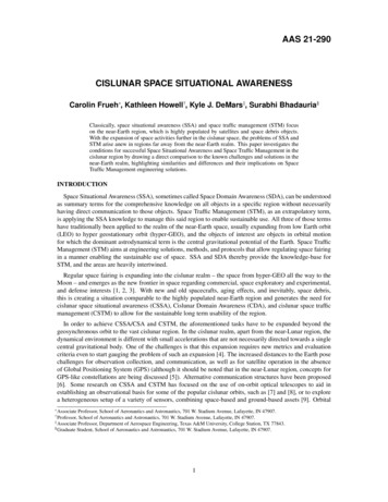
(a) Lyapunov Orbital Family, Rotating Frame(b) Selected Lyapunov orbit, Inertial FrameFigure 3: a) A family of L1 Lyapunov orbits in the Earth-Moon CR3BP. Colors indicate the energy range interms of the Jacobi Constant. One member of the family is selected (black) that passes relatively close to theMoon. b) the selected Lyapunov orbit propagated with the two different dynamical models (green simplifieddynamics, blue full ephemerides model) in the inertial J2000.0 frame.The Earth-L2 Halo Transfer OrbitTo investigate a different type of orbit in the cislunar regime, a transfer orbit is constructed from LEO toa three-dimensional L2 southern halo orbit [16, 17]. A projection of the transfer onto the x-y plane appearsin Fig. 4. The departure orbit is circular and 210 km altitude. The arrival L2 southern halo orbit possesses aperiod of 14.77 days; A member of the L2 halo family, the Jacobi constant value corresponding to this orbitis JC 3.13713. As apparent in the figure, the transfer includes two maneuvers, one to depart the Earth orbitand one to insert onto the halo orbit stable manifold. The Earth departure maneuver is quite standard; theinsertion maneuver at nearly 700 m/s has not been optimized and serves as a suitable initial guess for such atransfer. Consistent with the previous CR3BP orbits, the initial states for the transfer were straightforwardlyused in the two different dynamics models and propagated forward in time without any attempt to updatethe state prior to propagation and the resulting paths are plotted in Fig. 5. This is the resulting orbit withoutinclusion of the second maneuver. As a result, the orbit loops back to the Earth after the lunar passage.Employing a corrections process, the transfer would blend smoothly and, with a updated maneuver, flow intothe L2 orbit if this effort was focused upon a transfer. Rather, in this analysis, the path is employed to assesssurveillance capabilities; as such, the propagated arcs are sufficient.6

Figure 4: Transfer orbit between LEO and an L2 southern halo orbit in the Earth-Moon CR3BP.Figure 5: The selected Transfer orbit propagated with the two different dynamic models, simplified dynamicsand full ephemerides model in the inertial J2000.0 frame, just after the first maneuver.SURVEILLANCE OF THE SELECTED CISLUNAR ORBITSOne of the key elements in cislunar Space Surveillance is the coverage with observations. One of thechallenges are the large distances to the objects in the cislunar space. In this paper, the focus is on groundbased optical measurements. Those sensors are not the best suited ones, but the ones most widely available.For complete surveillance, supplementation of sensors on the Moon and on cislunar orbits are required.In order to model the optical sensor, the magnitude of a representative space object on the selected sampleorbits is computed. The magnitude of a space object is:mag magsun 2.5 log10 (Isc)Isun(5)where magsun is the apparent reference magnitude of the Sun, Isc is the irradiance reflected off the spacecraftand ISun is the Sun’s reference irradiance. In order to compute the irradiance that is reflected off the object,7

an assumption about the albedo-area, the shape and attitude of the space object has to be made. In this paper,we assume, in agreement with the solar radiation pressure modelling of a spherical object. This is a goodbaseline scenario. Overall, for satellites in a box wing configuration, higher irradiation is received in thecase of a specular glint off the solar panels or the antennas. However, those glints are, per definition, notcontinuous and only occur during very limited times over one period, if at all, depending on the Sun-objectobserver geometry. A Lambertian sphere on the other hand has the advantage of, other than in the time ofcomplete opposition, always reflecting a fraction of the Sun’s irradiation towards the observer; a fact notgiven for a non-spherical object. In future work, the exact orientation of a given satellite configuration willbe evaluated. The irradiance of the object can hence be expressed via the the following relation [18]:Isc ISun 2 Cd 2r (sin α (π α) cos α)d2scobs 3 π 2(6)dscobs is the distance between the object and the observer, r is the object’s radius, and α is the phase anglebetween the Sun and the observer at the object’s location. It is important to note that the solar constant I0 ,needs to be scaled to the actual distance between the Sun and the object dSunsc for the reference irradiance2as the solar constant is defined at one Astronomical Unit (AU). This is relevant whenISun I0 dAU2Sunsccomputing the absolute irradiation of the object.For the visibility besides the overall magnitude also the background irradiation entering the sensor arerelevant, creating the so-called detection signal to noise ratio (SNR) in its definition mean divided by thestandard deviation [19]:SNR S,S N(7)Where S and N denote the mean (and variance) of the Poisson distributed signal of interest and the noise,respectively. The signal of interest is in our case the signal contained in the object image on the detector andthe noise is in those same pixels.The detection limit is directly dependent on the SNR and is dictated by the exact setup of optic’s aperture,sensor type and sensitivity in combination with the specific image processing software. While, for methodologies employing stacking, detection limits can be pressed to be below an SNR of 1, this requires precisetracking and is inversely proportional to the time spent on observing the object, which is not realisticpor feasibile in many cases. In this paper, a realistic more general signal dependent threshold of SN R S/2 isused.Night time visibility constraints are often listed as a separate observation constraint, however, strictlyspeaking, night time constraints are also SNR constraints. Daytime imaging of satellites in off-Sun directionsis possible, however, the higher background requires a much higher object magnitude to reach the sameSNR. In general, daytime observations require magnitudes of 8 and brighter. In the investigations shownin this paper, none of the observation reached this magnitude, and brightest magnitudes are of the order of14 and higher. For this reason, night time constraintsare applied, requiring observations to take place afterpastronomical sunset. For the SNR a limit of S/2 is used, which serves as a lower bound.One of the most relevant background sources for cislunar observations is the lunar background, as observation directions close to the moon are more frequent. The lunar stray light is computed for each viewingdirection [20].Besides the SNR, visiblity constraints include, as the observations are assumed to be ground-based, localweather and local horizon constraints. The weather is highly variable and not taken into account here. A localhorizon constraint of 0 degrees above horizon has be employed, again serving as the lower limit.The Seleted DROFor the selected DRO orbit, Fig. 6 shows the magnitudes as a function of the time, measured from midnightJan 1, 2020 in hours, for various Cd values (see Eq. 6), local horizon constraints. The radius of the sphere8

is assumed to be 3.54 meters. The black bars indicate background night time sky’s moon brightness in theviewing direction to the object when observed from a station located at latitude 40.4310 degrees North andLongitude 86.9149 East. The gray bars indicate the night time, during which observations are possible. Thelowest magnitude is reached at all times, by the sphere with the highest reflectivity, of course. What is shownis that the moons background brightness significantly interferes with the observations from around 200 to 300hours. Overall, with a telescope with limiting magnitude of 16 only a fraction of the orbit can be covered withobservations even for the most reflective objects, at the beginning of the time interval and after 650 hours.Figure 6: The selected DRO: Magnitude of a 3.54 meter radius object as a function of time. The Skybrightness solely based on the Moon in the viewing direction is shown with the observation location at about40.4 deg N, 86.9 E.Figure 7: The selected DRO: Trajectory of the object and visibilities for a ground-based observer witha limiting magnitude of 20 and lunar background light, for a 1.8 meter radius object and Cd 0.5 anda minimum elevation of zero degrees. Ground-based sensor locations with visiblities are yellow, the oneswithout are marked in blue (Earth size not to scale), the trajectory, for which at least one ground-based sensorhas a visibility is marked pink, otherwise blue.9

The detectability of the object, not surprisingly, is highly dependent upon the location on the Earth, wherethe sensor is located. Fig. 7 shows the visibility of the DRO a 1.8 meter radius object with a reflection coefficient Cd 0.5, constrained to a zero elevation angle along withpmagnitude of the object that is larger thanthe Moon-induced background sky brightness with the SN R S/2 constraint and a limiting magnitudeof 20. The orbit which can be covered by observation located at the center of each Earth grid point is markedin pink and the corresponding sensor locations in yellow. Regions with no observation coverage by any earthsensor location is marked in black. More than in near-Earth surveillance, it is obvious a global network ofsensors is not optional. Furthermore, even with a global coverage, certain observation gaps exist, most significantly at regions after completing about half of the orbital period, in the region farthest from the earth.However, even when the object is closer, e.g. because of illumination conditions, visibility is not guaranteed,see Fig.7.The Selected Lyapunov OrbitFor the selected Lyapunov orbit, the same magnitude calculations have been performed for various Cdreflection coefficients for a spherical object with a radius of 3.54 meters, see Fig. 8. The ground-basedobserver has been placed again at latitude 40.4310 degrees North and Longitude 86.9149 degrees East.Shown are the night times via gray bars and the background moon light’s magnitude in the viewing directionto the object in black.Figure 8: The selected Lyapunov orbit: Magnitude of a one 3.54 meter radius object as a function of timewith the observation location at about 40.4 deg N, 86.9 deg E.Because the magnitude is largely dominated by the distance between the object and the observer, for asensor with a limiting magnitude of 16, one has only the early part of the trajectory to allow for observations,even with a sensor as sensitive as magnitude 20, only barely the last part of the orbit is allowed for observations. As the distance to the earth has significantly increased, no lower magnitudes are reached even for themost reflective objects. At the region, where the object is farthest from the earth, around 500 hours, in combination with the phase angle, no observations are possible, with the object becoming as faint as magnitude30. Towards the end of the propagation period, the object stays faint while also the moonlight thwarts anyobservation possibility. This is comparable to other sensor locations, as shown in Fig. 9.Fig. 9 shows the global visibility for a 1.8 meter radius object and a reflection coefficient Cd 0.5. Thevisiblity constraints are a limiting magnitude of 20, elevation constraints of 0 degrees local elevation anda magnitude of the objectp higher than the Moon-induced background sky brightness according to the SNRconstraint of SN R S/2 (compare Eq.7). Pink indicates visibility by at least one ground-based sensor,10

Figure 9: Trajectory of the object and visibilities for a ground-based observer with a limiting magnitudeof 20 and lunar background light, for a 1.8 meter radius object and Cd 0.5 and a minimum elevation ofzero degrees. Ground-based sensor locations with visiblities are yellow (none present at the final time, shownhere), the ones without are marked in blue (Earth size not to scale), the trajectory, for which at least oneground-based sensor has a visibility is marked pink, otherwise blue.black indicates no sensor can provide observations on the object. Sensors are located at the center of eachgrid point on the Earth surface. It is obvious that even with a ground-based sensor network of sensors withexcellent conditions (limiting magnitude 20), the object cannot be covered with observations towards the endof the propagation period. Observation coverage is reasonable up to this point. It can, however, again only beachieved with a global sensor network.The Selected Transfer OrbitThis can be compared to an object in the selected transfer orbit with the same spherical object with of3.54 meters radius, see Fig.10. with the same ground-based observer at latitude 40.4310 degrees North andLongitude 86.9149 degrees East. Shown are the night times via gray bars and the background moon light’smagnitude in the viewing direction to the object in black.Not surprisingly, the object is bright and very well to be observed at the times when it passes by the earth,however in the far lunar passages, the magnitude increases, making it impossible for sensors with a moderatelimiting magnitude to keep track of even this large object, especially when reflectivity i

Space Situational Awareness (SSA), sometimes called Space Domain Awareness (SDA), can be understood as summary terms for the comprehensive knowledge on all objects in a specific region without necessarily having direct communication to those objects.