Transcription
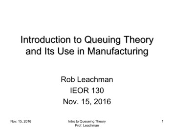
Introduction to Queuing Theoryand Its Use in ManufacturingRob LeachmanIEOR 130Nov. 15, 2016Nov. 15, 2016Intro to Queueing TheoryProf. Leachman1
Purpose In most service and production systems, thetime required to provide the service or tocomplete the product is important.– We may want to design and operate the system toachieve certain service standards. Generally, the time required includes “hands-on”time (actually processing) plus time waiting. Queuing theory is about the estimation of waitingtimes.Nov. 15, 2016Intro to Queueing TheoryProf. Leachman2
Terminology and Framework Customers arrive randomly for service and awaitavailability of a server– When the server(s) has (have) finished servicingprevious customers, the new customer can beginservice Time between arrival of customer and start ofservice is called the queue time Customer departs the system after completion ofthe service time Total time in system queue time service timeNov. 15, 2016Intro to Queueing TheoryProf. Leachman3
Analytical Approximation The mathematics of queuing theory is mucheasier if we assume the customer inter-arrivaltime has an exponential distribution, and if weassume the service time also has an exponentialdistribution. The exponential distribution has thememoryless property:– Suppose the average inter-arrival time is ta. Given ithas been t since the last customer arrival, what is theexpected time until the next customer arrival?Answer: Still ta !– Suppose the average service time is ts. Given it hasbeen t time units since service started, what is theexpected time until service ends? Answer: Still ts !Nov. 15, 2016Intro to Queueing TheoryProf. Leachman4
The M/M/1 Queue Queuing notation: A/B/n means inter-arrival timeshave distribution A, service times havedistribution B, n means there are n servers M means Markovian (memoryless), 1 means oneserver In a Markovian queuing system, the onlyinformation we need to characterize the state ofthe system is the number of customers n in thesystemNov. 15, 2016Intro to Queueing TheoryProf. Leachman5
The M/M/1 Queue (cont.) We write λ 1/ta as the arrival rate and µ 1/ts as the service rate. The utilization of the server is u ts/ta λ/µ. Note that we must have u 1 for thequeue to be stable.Nov. 15, 2016Intro to Queueing TheoryProf. Leachman6
The M/M/1 Queue (cont.) Markovian state-space: Node n represents thestate with n customers in the system The arcs show the rate at which the systemtransitions to an adjacent stateλ01µNov. 15, 201632µλλλµIntro to Queueing TheoryProf. Leachmanµ7
The M/M/1 Queue (cont.) Let pn probability system has n customers in it Because there is only one server, the systemcan only change by one unit at a time The system moves from state n to state n 1 atrate λ The system moves from state n 1 to state n atrate µ If the system is in a steady state, we must haveλpn µpn 1 or pn 1 (λ/µ) pn u pnNov. 15, 2016Intro to Queueing TheoryProf. Leachman8
The M/M/1 Queue (cont.)11 p n p0 u p 01 un 0n 0 Now So np0 1 u The expected total time a customer stays inthe system is n 0n 0n 0 ntnptptnputtnuu(1)(1) s s 0 sns ns nn 0 t s t s n(1 u )u t s t s (1 u )u nu n 1nn 0n 0d nd nu t s t s (1 u )u u t s t s (1 u )u du n 0n 0 du Nov. 15, 2016tsd 1 u t s t s (1 u )u ts tsdu 1 u (1 u ) (1 u )Intro to Queueing TheoryProf. Leachman9
The M/M/1 Queue (cont.) And so the expected queue time istsuQT ts ts .1 u1 uNov. 15, 2016Intro to Queueing TheoryProf. Leachman10
Numerical Example Suppose ts 12 minutes, λ 4 per hour Then u λ/µ λ* ts 4 (12/60) 80% Probability server is idle 1 – u 20%ut s (0.8/0.2)*(12) Expected queue time 1 u48 minutes Expected time in system 48 12 60 minutesNov. 15, 2016Intro to Queueing TheoryProf. Leachman11
Queuing in Manufacturing Customers production lots. Total time a lot is ata production step (wait process) is called thecycle time of the step. Servers machines. Machines requiremaintenance. They are only available forprocessing work part of the time. Suppose the availability is A and the processtime is PT. The effective long-run service rate isµ A * (1/PT). u becomes u λ/µ λ (PT / A). Note that we decrease the service rate and weincrease utilization to account for machine downtimeNov. 15, 2016Intro to Queueing TheoryProf. Leachman12
Queuing in Manufacturing (cont.) When we have one machine, we can estimateu PTthe avg. queue time as: QT 1 u A Queuing model: Time in system queue time PTservice time QT A Real life: Time in system wait time processtime (wait time) PTPT PT QT ts PT So (wait time) QT ANov. 15, 2016Intro to Queueing TheoryProf. Leachman13
Queuing in Manufacturing (cont.) The standard cycle time SCT is the total time alot is resident at the production step when thereis no waiting. It is often somewhat larger thanthe process time PT as it accounts for materialhandling time or other factors performed inparallel with the processing of other lots. Therefore, lot CT (wait time) SCT (QT ts – PT) SCT QT (1/A – 1)PT SCTNov. 15, 2016Intro to Queueing TheoryProf. Leachman14
Queuing in Manufacturing (cont.) Another way to think of this is:(Cycle time) (Time in queuing system) (portion of cycle time not in queuing system) (QT PT / A) SCT – PT QT (1/A – 1)*PT SCTNov. 15, 2016Intro to Queueing TheoryProf. Leachman15
Numerical example Availability of machine A 85% Arrival rate of lots λ 2 per hour PT 0.25 hours (i.e., 15 minutes), SCT 0.30hours (i.e., 18 minutes) u (2)(0.25)/0.85 0.588 QT [0.588/(1-0.588)]*(0.25/0.85) 0.42 hours 25 minutes CT 25 (1/0.85 -1)*15 18 45.6 minutes Note that the avg. waiting time (30.6 mins) ismuch longer than the process time (15 mins)Nov. 15, 2016Intro to Queueing TheoryProf. Leachman16
More general queuing formula We may have m machines instead of 1 Service and arrival rates might not be exponential,machines may experience long down times (failures ormajor maintenance events) Generic formula for queue time per lot or batch(Kingman, Sakasegawa, Hopp and Spearman): ca 2 ce 2 u 2 ( m 1) 1 PT QT 2 m(1 u ) A Nov. 15, 2016Intro to Queueing TheoryProf. Leachman17
More general formula (cont.) ca2 is the normalized variance (the squaredcoefficient of variation, or “c.v.2” for short) of thearrival rate, i.e., ca2 σa2/λ2 ce2 is the normalized variance of the (effective)service time, composed of the following: c02 is the normalized variance of the processtime, i.e., c02 σPT2/PT2 MTTR is the average length of a downtime event cr2 is the normalized variance of the length of anequipment-down event, i.e., cr2 σr2/MTTR2Nov. 15, 2016Intro to Queueing TheoryProf. Leachman18
More general formula (cont.) A is the average availability of the machine type Then MTTR ce c (1 cr ) A(1 A) PT 2Nov. 15, 2016202Intro to Queueing TheoryProf. Leachman19
Queuing Analysis (cont.)Key point: Wait time (u ) 2( m 1) 1{Variability} { m(1 u ) } {Process time/Availability} {Process time} {1/Availability – 1} One can reduce cycle time if any of the aboveterms is reduced (i.e., reduce variability, reduceu, increase m, reduce PT, or increase A)Nov. 15, 2016Intro to Queueing TheoryProf. Leachman20
Queuing Analysis (cont.){Variability} ce effective service time c.v. (reflectsmachine down time)– Let c0 denote intrinsic process time c.v., cr denoterepair time c.v., A denote availability, MTTR denotemean time to repair, PT denote avg. process timeMTTRkce c (1 cr ) Ak (1 Ak )PTk2k202kUtilization should be kept lower for machines with highervariabilityNov. 15, 2016Intro to Queueing TheoryProf. Leachman21
Queuing Analysis (cont.){Utilization} System performance is very sensitive to high utilization levels.Wait Time vs. Utilization109876543210Wait Time (1 machine)Wait Time (2 machines)Wait Time (3 50.30.350.20.25Wait Time (8 machines)0.10.150.05 Increasing thenumber of qualifiedmachines reduceswait time:Wait Time Balancing utilizationreduces wait time.UtilizationNov. 15, 2016Intro to Queueing TheoryProf. Leachman22
a production step (wait process) is called the cycle time of the step. Servers machines. Machines require maintenance. They are only available for processing work part of the time. Suppose the availability is A and the process time is PT. The effective long-run service