WIXLIB

1INTRODUCTION TO INFORMATION THEORY{ch:intro info}This chapter introduces some of the basic concepts of information theory, as wellas the definitions and notations of probabilities that will be used throughoutthe book. The notion of entropy, which is fundamental to the whole topic ofthis book, is introduced here. We also present the main questions of informationtheory, data compression and error correction, and state Shannon’s theorems.1.1Random variablesThe main object of this book will be the behavior of large sets of discreterandom variables. A discrete random variable X is completely defined1 bythe set of values it can take, X , which we assume to be a finite set, and itsprobability distribution {pX (x)}x X . The value pX (x) is the probability thatthe random variable X takes the value x. The probability distribution pX : X [0, 1] must satisfy the normalization conditionXpX (x) 1 .(1.1)x XWe shall denote by P(A) the probability of an event A X , so that pX (x) P(X x). To lighten notations, when there is no ambiguity, we use p(x) todenote pX (x).If f (X) is a real valued function of the random variable X, the expectationvalue of f (X), which we shall also call the average of f , is denoted by:Ef XpX (x)f (x) .(1.2)x XWhile our main focus will be on random variables taking values in finitespaces, we shall sometimes make use of continuous random variables takingvalues in Rd or in some smooth finite-dimensional manifold. The probabilitymeasure for an ‘infinitesimal element’ dx will be denoted by dpX (x). Each timepX admits a density (with respect to the Lebesgue measure), we shall use thenotation pX (x) for the value of this density at the point x. The total probabilityP(X A) that the variable X takes value in some (Borel) set A X is givenby the integral:1 In probabilistic jargon (which we shall avoid hereafter), we take the probability spaceP(X , P(X ), pX ) where P(X ) is the σ-field of the parts of X and pX x X pX (x) δx .1{proba norm}

2INTRODUCTION TO INFORMATION THEORYP(X A) ZdpX (x) x AZI(x A) dpX (x) ,(1.3)where the second form uses the indicator function I(s) of a logical statements,which is defined to be equal to 1 if the statement s is true, and equal to 0 ifthe statement is false.The expectation value of a real valued function f (x) is given by the integralon X :ZE f (X) f (x) dpX (x) .(1.4)Sometimes we may write EX f (X) for specifying the variable to be integratedover. We shall often use the shorthand pdf for the probability density function pX (x).Example 1.1 A fair dice with M faces has X {1, 2, ., M } and p(i) 1/Mfor all i {1, ., M }. The average of x is E X (1 . M )/M (M 1)/2.Example 1.2 Gaussian variable: a continuous variable X R has a Gaussiandistribution of mean m and variance σ 2 if its probability density is 1[x m]2.(1.5)p(x) exp 2σ 22πσOne has EX m and E(X m)2 σ 2 .The notations of this chapter mainly deal with discrete variables. Most of theexpressionscan be transposed to the case of continuous variables by replacingPsums x by integrals and interpreting p(x) as a probability density.Exercise 1.1 Jensen’s inequality. Let X be a random variable taking valuein a set X R and f a convex function (i.e. a function such that x, y and α [0, 1]: f (αx (1 αy)) αf (x) (1 α)f (y)). ThenEf (X) f (EX) .{eq:Jensen}(1.6)Supposing for simplicity that X is a finite set with X n, prove this equalityby recursion on n.{se:entropy}1.2EntropyThe entropy HX of a discrete random variable X with probability distributionp(x) is defined as X1{S def},(1.7)HX p(x) log2 p(x) E log2p(X)x X

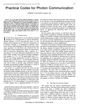
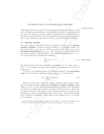
ENTROPY3where we define by continuity 0 log2 0 0. We shall also use the notation H(p)whenever we want to stress the dependence of the entropy upon the probabilitydistribution of X.In this Chapter we use the logarithm to the base 2, which is well adaptedto digital communication, and the entropy is then expressed in bits. In othercontexts one rather uses the natural logarithm (to base e 2.7182818). It issometimes said that, in this case, entropy is measured in nats. In fact, the twodefinitions differ by a global multiplicative constant, which amounts to a changeof units. When there is no ambiguity we use H instead of HX .Intuitively, the entropy gives a measure of the uncertainty of the randomvariable. It is sometimes called the missing information: the larger the entropy,the less a priori information one has on the value of the random variable. Thismeasure is roughly speaking the logarithm of the number of typical values thatthe variable can take, as the following examples show.Example 1.3 A fair coin has two values with equal probability. Its entropy is1 bit.Example 1.4 Imagine throwing M fair coins: the number of all possible outcomes is 2M . The entropy equals M bits.Example 1.5 A fair dice with M faces has entropy log2 M .Example 1.6 Bernouilli process. A random variable X can take values 0, 1with probabilities p(0) q, p(1) 1 q. Its entropy isHX q log2 q (1 q) log2 (1 q) ,(1.8){S bern}it is plotted as a function of q in fig.1.1. This entropy vanishes when q 0or q 1 because the outcome is certain, it is maximal at q 1/2 when theuncertainty on the outcome is maximal.Since Bernoulli variables are ubiquitous, it is convenient to introduce thefunction H(q) q log q (1 q) log(1 q), for their entropy.Exercise 1.2 An unfair dice with four faces and p(1) 1/2, p(2) 1/4, p(3) p(4) 1/8 has entropy H 7/4, smaller than the one of thecorresponding fair dice.‘‘Info Phys Comp’’ Draft: November 9, 2007 -- ‘‘Info Phys

4INTRODUCTION TO INFORMATION .40.50.60.70.80.91qFig. 1.1. The entropy H(q) of a binary variable with p(X 0) q,p(X 1) 1 q, plotted versus q{fig bernouilli}Exercise 1.3 DNA is built from a sequence of bases which are of four types,A,T,G,C. In natural DNA of primates, the four bases have nearly the samefrequency, and the entropy per base, if one makes the simplifying assumptionsof independence of the various bases, is H log2 (1/4) 2. In some genus ofbacteria, one can have big differences in concentrations: p(G) p(C) 0.38,p(A) p(T ) 0.12, giving a smaller entropy H 1.79.Exercise 1.4 In some intuitive way, the entropy of a random variable is relatedto the ‘risk’ or ‘surprise’ which are associated to it. In this example we discussa simple possibility for making these notions more precise.Consider a gambler who bets on a sequence of bernouilli random variablesXt {0, 1}, t {0, 1, 2, . . . } with mean EXt p. Imagine he knows thedistribution of the Xt ’s and, at time t he bets a fraction w(1) p of his moneyon 1 and a fraction w(0) (1 p) on 0. He looses whatever is put on the wrongnumber, while he doubles whatever has been put on the right one. Define theaverage doubling rate of his wealth at time t as( t)Y1Wt E log22w(Xt′ ) .(1.9)t′t 1It is easy to prove that the expected doubling rate EWt is related to the entropyof Xt : EWt 1 H(p). In other words, it is easier to make money out ofpredictable events.Another notion that is directly related to entropy is the Kullback-Leibler‘‘Info Phys Comp’’ Draft: November 9, 2007 -- ‘‘Info Phys

ENTROPY5(KL) divergence between two probability distributions p(x) and q(x) over thesame finite space X . This is defined as:D(q p) Xx Xq(x) logq(x)p(x)(1.10)where we adopt the conventions 0 log 0 0, 0 log(0/0) 0. It is easy to showthat: (i) D(q p) is convex in q(x); (ii) D(q p) 0; (iii) D(q p) 0 unlessq(x) p(x). The last two properties derive from the concavity of the logarithm(i.e. the fact that the function log x is convex) and Jensen’s inequality (1.6):if E denotes expectation with respect to the distribution q(x), then D(q p) E log[p(x)/q(x)] log E[p(x)/q(x)] 0. The KL divergence D(q p) thus lookslike a distance between the probability distributions q and p, although it is notsymmetric.The importance of the entropy, and its use as a measure of information,derives from the following properties:1. HX 0.2. HX 0 if and only if the random variable X is certain, which means thatX takes one value with probability one.3. Among all probability distributions on a set X with M elements, H ismaximum when all events x are equiprobable, with p(x) 1/M . Theentropy is then HX log2 M .Notice in fact that, if X has M elements, then the KL divergence D(p p)between p(x) and the uniform distribution p(x) 1/M is D(p p) log2 M H(p). The thesis follows from the properties of the KL divergence mentioned above.4. If X and Y are two independent random variables, meaning that pX,Y (x, y) pX (x)pY (y), the total entropy of the pair X, Y is equal to HX HY :HX,Y Xp(x, y) log2 pX,Y (x, y) x,yXpX (x)pY (y) (log2 pX (x) log2 pY (y)) HX HY(1.11)x,y5. For any pair of random variables, one has in general HX,Y HX HY ,and this result is immediately generalizable to n variables. (The proof can be obtained by using the positivity of the KL divergence D(p1 p2 ), wherep1 pX,Y and p2 pX pY ).6. Additivity for composite events. Take a finite set of events X , Pand decompose it into X X1 X2 , where X1 X2 . Call q1 x X1 p(x)the probability of X1 , and q2 the probability of X2 . For each x X1 ,define as usual the conditional probability of x, given that x X1 , byr1 (x) p(x)/q1 and define similarly r2 (x) as the conditional probability‘‘Info Phys Comp’’ Draft: November 9, 2007 -- ‘‘Info Phys

6INTRODUCTION TO INFORMATION THEORYof x, given that x X2 . Then Pthe total entropy can be written as the sumof two contributions HX x X p(x) log2 p(x) H(q) H(r), where:H(q) q1 log2 q1 q2 log2 q2XXr2 (x) log2 r2 (x)r1 (x) log2 r1 (x) q2H(r) q1{sec:RandomVarSequences}(1.13)x X1x X1 (1.12)The proof is obvious by just substituting the laws r1 and r2 by their expanded definitions. This property is interpreted as the fact that the averageinformation associated to the choice of an event x is additive, being thesum of the relative information H(q) associated to a choice of subset, andthe information H(r) associated to the choice of the event inside the subsets (weighted by the probability of the subsetss). It is the main propertyof the entropy, which justifies its use as a measure of information. In fact,this is a simple example of the so called chain rule for conditional entropy,which will be further illustrated in Sec. 1.4.Conversely, these properties together with some hypotheses of continuity andmonotonicity can be used to define axiomatically the entropy.1.3Sequences of random variables and entropy rateIn many situations of interest one deals with a random process which generatessequences of random variables {Xt }t N , each of them taking values in thesame finite space X . We denote by PN (x1 , . . . , xN ) the joint probability distribution of the first N variables. If A {1, . . . , N } is a subset of indices, weshall denote by A its complement A {1, . . . , N } \ A and use the notationsxA {xi , i A} and xA {xi , i A}. The marginal distribution of thevariables in A is obtained by summing PN on the variables in A:PA (xA ) XPN (x1 , . . . , xN ) .(1.14)xAExample 1.7 The simplest case is when the Xt ’s are independent. Thismeans that PN (x1 , . . . , xN ) p1 (x1 )p2 (x2 ) . . . pN (xN ). If all the distributionspi are identical, equal to p, the variables are independent identically distributed, which will be abbreviated as iid. The joint distribution isPN (x1 , . . . , xN ) NYp(xi ) .(1.15)t 1‘‘Info Phys Comp’’ Draft: November 9, 2007 -- ‘‘Info Phys