Transcription
Philosophy and the practice of Bayesian statisticsAndrew GelmanDepartment of Statistics and Department of Political Science, Columbia UniversityCosma Rohilla ShaliziStatistics Department, Carnegie Mellon UniversitySanta Fe Institute27 June 2011AbstractA substantial school in the philosophy of science identifies Bayesian inference withinductive inference and even rationality as such, and seems to be strengthened by therise and practical success of Bayesian statistics. We argue that the most successfulforms of Bayesian statistics do not actually support that particular philosophy butrather accord much better with sophisticated forms of hypothetico-deductivism. Weexamine the actual role played by prior distributions in Bayesian models, and the crucialaspects of model checking and model revision, which fall outside the scope of Bayesianconfirmation theory. We draw on the literature on the consistency of Bayesian updatingand also on our experience of applied work in social science.Clarity about these matters should benefit not just philosophy of science, but alsostatistical practice. At best, the inductivist view has encouraged researchers to fit andcompare models without checking them; at worst, theorists have actively discouragedpractitioners from performing model checking because it does not fit into their framework.1The usual story—which we don’t likeIn so far as I have a coherent philosophy of statistics, I hope it is “robust” enoughto cope in principle with the whole of statistics, and sufficiently undogmatic notto imply that all those who may think rather differently from me are necessarilystupid. If at times I do seem dogmatic, it is because it is convenient to give myown views as unequivocally as possible. (Bartlett, 1967, p. 458)Schools of statistical inference are sometimes linked to approaches to the philosophyof science. “Classical” statistics—as exemplified by Fisher’s p-values, Neyman-Pearsonhypothesis tests, and Neyman’s confidence intervals—is associated with the hypotheticodeductive and falsificationist view of science. Scientists devise hypotheses, deduce implications for observations from them, and test those implications. Scientific hypotheses can berejected (that is, falsified), but never really established or accepted in the same way. Mayo(1996) presents the leading contemporary statement of this view.1
In contrast, Bayesian statistics or “inverse probability”—starting with a prior distribution, getting data, and moving to the posterior distribution—is associated with an inductiveapproach of learning about the general from particulars. Rather than testing and attemptedfalsification, learning proceeds more smoothly: an accretion of evidence is summarized by aposterior distribution, and scientific process is associated with the rise and fall in the posterior probabilities of various models; see Figure 1 for a schematic illustration. In this view,the expression p(θ y) says it all, and the central goal of Bayesian inference is computingthe posterior probabilities of hypotheses. Anything not contained in the posterior distribution p(θ y) is simply irrelevant, and it would be irrational (or incoherent) to attemptfalsification, unless that somehow shows up in the posterior. The goal is to learn aboutgeneral laws, as expressed in the probability that one model or another is correct. Thisview, strongly influenced by Savage (1954), is widespread and influential in the philosophyof science (especially in the form of Bayesian confirmation theory; see Howson and Urbach1989; Earman 1992) and among Bayesian statisticians (Bernardo and Smith, 1994). Manypeople see support for this view in the rising use of Bayesian methods in applied statisticalwork over the last few decades.1We think most of this received view of Bayesian inference is wrong.2 Bayesian methodsare no more inductive than any other mode of statistical inference. Bayesian data analysisis much better understood from a hypothetico-deductive perspective.3 Implicit in the bestBayesian practice is a stance that has much in common with the error-statistical approach ofMayo (1996), despite the latter’s frequentist orientation. Indeed, crucial parts of Bayesiandata analysis, such as model checking, can be understood as “error probes” in Mayo’s sense.We proceed by a combination of examining concrete cases of Bayesian data analysis in1Consider the current (9 June 2010) state of the Wikipedia article on Bayesian inference, which begins asfollows:Bayesian inference is statistical inference in which evidence or observations are used to updateor to newly infer the probability that a hypothesis may be true.It then continues with:Bayesian inference uses aspects of the scientific method, which involves collecting evidence thatis meant to be consistent or inconsistent with a given hypothesis. As evidence accumulates,the degree of belief in a hypothesis ought to change. With enough evidence, it should becomevery high or very low. . . . Bayesian inference uses a numerical estimate of the degree of beliefin a hypothesis before evidence has been observed and calculates a numerical estimate ofthe degree of belief in the hypothesis after evidence has been observed. . . . Bayesian inferenceusually relies on degrees of belief, or subjective probabilities, in the induction process and doesnot necessarily claim to provide an objective method of induction. Nonetheless, some Bayesianstatisticians believe probabilities can have an objective value and therefore Bayesian inferencecan provide an objective method of induction.These views differ from those of, e.g., Bernardo and Smith (1994) or Howson and Urbach (1989) only in theomission of technical details.2We are claiming that most of the standard philosophy of Bayes is wrong, not that most of Bayesianinference itself is wrong. A statistical method can be useful even if its philosophical justification is in error.It is precisely because we believe in the importance and utility of Bayesian inference that we are interestedin clarifying its foundations.3We are not interested in the hypothetico-deductive “confirmation theory” prominent in philosophy ofscience from the 1950s through the 1970s, and linked to the name of Hempel (1965). The hypotheticodeductive account of scientific method to which we appeal is distinct from, and much older than, thisparticular sub-branch of confirmation theory.2
Figure 1: Hypothetical picture of idealized Bayesian inference under the conventional inductive philosophy. The posterior probability of different models changes over time withthe expansion of the likelihood as more data are entered into the analysis. Depending onthe context of the problem, the time scale on the x-axis might be hours, years, or decades,in any case long enough for information to be gathered and analyzed that first knocks outhypothesis 1 in favor of hypothesis 2, which in turn is dethroned in favor of the currentchampion, model 3.empirical social science research, and theoretical results on the consistency and convergenceof Bayesian updating. Social-scientific data analysis is especially salient for our purposesbecause there is general agreement that, in this domain, all models in use are wrong—notmerely falsifiable, but actually false. With enough data—and often only a fairly moderateamount—any analyst could reject any model now in use to any desired level of confidence.Model fitting is nonetheless a valuable activity, and indeed the crux of data analysis. Tounderstand why this is so, we need to examine how models are built, fitted, used, andchecked, and the effects of misspecification on models.Our perspective is not new; in methods and also in philosophy we follow statisticianssuch as Box (1980, 1983, 1990), Good and Crook (1974), Good (1983), Morris (1986), Hill(1990), and Jaynes (2003). All these writers emphasized the value of model checking andfrequency evaluation as guidelines for Bayesian inference (or, to look at it another way,the value of Bayesian inference as an approach for obtaining statistical methods with goodfrequency peroperties; see Rubin 1984). Despite this literature, and despite the strongthread of model checking in applied statistics, this philosophy of Box and others remains aminority view that is much less popular than the idea of Bayes being used to update theprobabilities of different candidate models being true (as can be seen, for example, by theWikipedia snippets given in footnote 1).A puzzle then arises: The evidently successful methods of modeling and model checking (associated with Box, Rubin, and others) seems out of step with the accepted view ofBayesian inference as inductive reasoning (what we call here “the usual story”)? How can weunderstand this disjunction? One possibility (perhaps held by the authors of the Wikipediaarticle) is that the inductive-Bayes philosophy is correct and that the model-building approach of Box et al. can, with care, be interpreted in that way. Another possibility is that3
the approach characterized by Bayesian model checking and continuous model expansioncould be improved by moving to a fully-Bayesian approach centering on the posterior probabilities of competing models. A third possibility, which we advocate, is that Box, Rubin,et al. are correct and that the usual philosophical story of Bayes as inductive inference isfaulty.We are interested in philosophy and think it is important for statistical practice—if nothing else, we believe that strictures derived from philosophy can inhibit research progress.4That said, we are statisticians, not philosophers, and we recognize that our coverage of thephilosophical literature will be incomplete. In this presentation, we focus on the classicalideas of Popper and Kuhn, partly because of their influence in the general scientific culture and partly because they represent certain attitudes which we believe are important inunderstanding the dynamic process of statistical modeling. We also emphasize the workof Mayo (1996) and Mayo and Spanos (2006) because of its relevance to our discussion ofmodel checking. We hope and anticipate that others can expand the links to other modernstrands of philosophy of science such as Giere (1988); Haack (1993); Kitcher (1993); Laudan(1996) which are relevant to the freewheeling world of practical statistics; our goal here isto demonstrate a possible Bayesian philosophy that goes beyond the usual inductivism andcan better match Bayesian practice as we know it.2The data-analysis cycleWe begin with a very brief reminder of how statistical models are built and used in dataanalysis, following Gelman et al. (2003), or, from a frequentist perspective, Guttorp (1995).The statistician begins with a model that stochastically generates all the data y, whosejoint distribution is specified as a function of a vector of parameters θ from a space Θ(which may, in the case of some so-called non-parametric models, be infinite dimensional).This joint distribution is the likelihood function. The stochastic model may involve other,unmeasured but potentially observable variables ỹ—that is, missing or latent data—andmore-or-less fixed aspects of the data-generating process as covariates. For both Bayesiansand frequentists, the joint distribution of (y, ỹ) depends on θ. Bayesians insist on a full jointdistribution, embracing observables, latent variables, and parameters, so that the likelihoodfunction becomes a conditional probability density, p(y θ). In designing the stochastic process for (y, ỹ), the goal is to represent the systematic relationships between the variablesand between the variables and the parameters, and as well as to represent the noisy (contingent, accidental, irreproducible) aspects of the data stochastically. Against the desirefor accurate representation one must balance conceptual, mathematical and computationaltractability. Some parameters thus have fairly concrete real-world referents, such as the famous (in statistics) survey of the rat population of Baltimore (Brown et al., 1955). Others,however, will reflect the specification as a mathematical object more than the reality being modeled—t-distributions are sometimes used to model heavy-tailed observational noise,with the number of degrees of freedom for the t representing the shape of the distribution;few statisticians would take this as realistically as the number of rats.4For example, we have more than once encountered Bayesian statisticians who had no interest in assessingthe fit of their models to data because they felt that Bayesian models were by definition subjective, and thusneither could nor should be tested.4
Bayesian modeling, as mentioned, requires a joint distribution for (y, ỹ, θ), which isconveniently factored (without loss of generality) into a prior distributionfor the parameRters, p(θ), and the complete-data likelihood, p(y, ỹ θ), so that p(y θ) p(y, ỹ θ)dỹ. Theprior distribution is, as we will see, really part of the model. In practice, the various partsof the model have functional forms picked by a mix of substantive knowledge, scientificconjectures, statistical properties, analytical convenience, disciplinary tradition, and computational tractability.Having completed the specification, the Bayesian analyst calculates the posterior distribution p(θ y); it is so that this quantity makes sense that the observed y and the parametersθ must have a joint distribution. The rise of Bayesian methods in applications has restedon finding new ways of to actually carry through this calculation, even if only approximately, notably by adopting Markov chain Monte Carlo methods, originally developed instatistical physics to evaluate high-dimensional integrals (Metropolis et al., 1953; Newmanand Barkema, 1999), to sample from the posterior distribution. The natural counterpart ofthis stage for non-Bayesian analyses are various forms of point and interval estimation toidentify the set of values of θ that are consistent with the data y.According to the view we sketched above, data analysis basically ends with the calculation of the posterior p(θ y). At most, this might be elaborated by partitioning Θ into a setof models or hypotheses, Θ1 , .ΘK , each with a prior probability p(Θk ) and its own set ofparameters θk . One would then compute the posterior parameter distribution within eachmodel, p(θk y, Θk ), and the posterior probabilities of the models,p(Θk y) p(Θk )p(y Θk )k0 (p(Θk0 )p(y Θk0 ))Rp(Θk ) p(y, θk Θk )dθkRP.k0 (p(Θk0 ) p(y, θk Θk0 )dθk0 )PThese posterior probabilities of hypotheses can be used for Bayesian model selection orBayesian model averaging (topics to which we return below). Scientific progress, in thisview, consists of gathering data—perhaps through well-designed experiments, designed todistinguish among interesting competing scientific hypotheses (cf. Atkinson and Donev,1992; Paninski, 2005)—and then plotting the p(Θk y)’s over time and watching the systemlearn (as sketched in Figure 1).In our view, the account of the last paragraph is crucially mistaken. The data-analysisprocess—Bayesian or otherwise—does not end with calculating parameter estimates or posterior distribution. Rather, the model can then be checked, by comparing the implicationsof the fitted model to the empirical evidence. One asks questions like, Do simulations fromthe fitted model resemble the original data? Is the fitted model consistent with other datanot used in the fitting of the model? Do variables that the model says are noise (“errorterms”) in fact display readily-detectable patterns? Discrepancies between the model anddata can be used to learn about the ways in which the model is inadequate for the scientificpurposes at hand, and thus to motivate expansions and changes to the model (§4).5
Figure 2: Based on a model fitted to survey data: states won by John McCain and BarackObama among different ethnic and income categories. States colored deep red and deep blueindicate clear McCain and Obama wins; pink and light blue represent wins by narrowermargins, with a continuous range of shades going to gray for states estimated at exactly50/50. The estimates shown here represent the culmination of months of effort, in whichwe fit increasingly complex models, at each stage checking the fit by comparing to data andthen modifying aspects of the prior distribution and likelihood as appropriate.6
Figure 3: Some of the data and fitted model used to make the maps shown in Figure 2.Dots are weighted averages from pooled June-November Pew surveys; error bars show 1standard error bounds. Curves are estimated using multilevel models and have a standarderror of about 3% at each point. States are ordered in decreasing order of McCain vote(Alaska, Hawaii, and D.C. excluded). We fit a series of models to these data; only this lastmodel fit the data well enough that we were satisfied. In working with larger datasets andstudying more complex questions, we encounter increasing opportunities to check model fitand thus falsify in a way that is helpful for our research goals.7
2.1Example: Estimating voting patterns in subsets of the populationWe demonstrate the hypothetico-deductive Bayesian modeling process with an examplefrom our recent applied research (Gelman et al., 2010). In recent years, American politicalscientists have been increasingly interested in the connections between politics and incomeinequality (see, e.g., McCarty et al. 2006). In our own contribution to this literature, weestimated the attitudes of rich, middle-income, and poor voters in each of the fifty states(Gelman et al., 2008b). As we described in our article on the topic (Gelman et al., 2008c),we began by fitting a varying-intercept logistic regression: modeling votes (coded as y 1for votes for the Republican presidential candidate or y 0 for Democratic votes) givenfamily income (coded in five categories from low to high as x 2, 1, 0, 1, 2), using amodel of the form Pr (y 1) logit 1 (as bx), where s indexes state of residence—themodel is fit to survey responses—and the varying intercepts as correspond to some statesbeing more Republican-leaning than others. Thus, for example as has a positive value in aconservative state such as Utah and a negative value in a liberal state such as California.The coefficient b represents the “slope” of income, and its positive value indicates that,within any state, richer voters are more likely to vote Republican.It turned out that this varying-intercept model did not fit our data, as we learnedby making graphs of the average survey response and fitted curves for the different incomecategories within each state. We had to expand to a varying-intercept, varying-slope model,Pr (y 1) logit 1 (as bs x), in which the slopes bs varied by state as well. This modelexpansion led to a corresponding expansion in our understanding: we learned that the gapin voting between rich and poor is much greater in poor states such as Mississippi than inrich states such as Connecticut. Thus, the polarization between rich and poor voters variedin important ways geographically.We found this not through any process of Bayesian induction but rather through modelchecking. Bayesian inference was crucial, not for computing the posterior probability thatany particular model was true—we never actually did that—but in allowing us to fit richenough models in the first place that we could study state-to-state variation, incorporatingin our analysis relatively small states such as Mississippi and Connecticut that did not havelarge samples in our survey. (Gelman and Hill 2006 review the hierarchical models thatallow such partial pooling.)Life continues, though, and so do our statistical struggles. After the 2008 election,we wanted to make similar plots, but this time we found that even our more complicatedlogistic regression model did not fit the data—especially when we wanted to expand ourmodel to estimate voting patterns for different ethnic groups. Comparison of data to fitled to further model expansions, leading to our current specification, which uses a varyingintercept, varying-slope logistic regression as a baseline but allows for nonlinear and evennon-monotonic patterns on top of that. Figure 2 shows some of our inferences in map form,while Figure 3 shows one of our diagnostics of data and model fit.The power of Bayesian inference here is deductive: given the data and some modelassumptions, it allows us to make lots of inferences, many of which can be checked andpotentially falsified. For example, look at New York state (in the bottom row of Figure 3):apparently, voters in the second income category supported John McCain much more thandid voters in neighboring income groups in that state. This pattern is theoretically possible8
but it arouses suspicion. A careful look at the graph reveals that this is a pattern in theraw data which was moderated but not entirely smoothed away by our model. The naturalnext step would be to examine data from other surveys. We may have exhausted what wecan learn from this particular dataset, and Bayesian inference was a key tool in allowing usto do so.3The Bayesian principal-agent problemBefore returning to discussions of induction and falsification, we briefly discuss some findingsrelating to Bayesian inference under misspecified models. The key idea is that Bayesianinference for model selection—statements about the posterior probabilities of candidatemodels—does not solve the problem of learning from data about problems with existingmodels.In economics, the “principal-agent problem” refers to the difficulty of designing contractsor institutions which ensure that one selfish actor, the “agent,” will act in the interests ofanother, the “principal,” who cannot monitor and sanction their agent without cost orerror. The problem is one of aligning incentives, so that the agent serves itself by servingthe principal (Eggertsson, 1990). There is, as it were, a Bayesian principal-agent problem aswell. The Bayesian agent is the methodological fiction (now often approximated in software)of a creature with a prior distribution over a well-defined hypothesis space Θ, a likelihoodfunction p(y θ), and conditioning as its sole mechanism of learning and belief revision. Theprincipal is the actual statistician or scientist.The Bayesian agent’s ideas are much more precise than the actual scientist’s; in particular, the Bayesian (in this formulation, with which we disagree) is certain that some θis the exact and complete truth, whereas the scientist is not.5 At some point in history,a statistician may well write down a model which he or she believes contains all the systematic influences among properly-defined variables for the system of interest, with correctfunctional forms and distributions of noise terms. This could happen, but we have neverseen it, and in social science we’ve never seen anything that comes close, either. If nothingelse, our own experience suggests that however many different specifications we think of,there are always others which had not occurred to us, but cannot be immediately dismisseda priori, if only because they can be seen as alternative approximations to the ones wemade. Yet the Bayesian agent is required to start with a prior distribution whose supportcovers all alternatives that could be considered.6This is not a small technical problem to be handled by adding a special value of θ, say θ standing for “none of the above”; even if one could calculate p(y θ ), the likelihood of thedata under this catch-all hypothesis, this in general would not lead to just a small correctionto the posterior, but rather would have substantial effects (Fitelson and Thomason, 2008).5In claiming that “the Bayesian” is certain that some θ is the exact and complete truth, we are notclaiming that actual Bayesian scientists or statisticians hold this view. Rather, we are saying that this isimplied by the philosophy we are attacking here. All statisticians, Bayesian and otherwise, recognize thatthe philosophical position which ignores this approximation is problematic.6It is also not at all clear that Savage and other founders of Bayesian decision theory ever thought thatthis principle should apply outside of the small worlds of artificially simplified and stylized problems—seeBinmore (2007). But as scientists we care about the real, large world.9
Fundamentally, the Bayesian agent is limited by the fact that its beliefs always remainwithin the support of its prior. For the Bayesian agent, the truth must, so to speak, bealways already partially believed before it can become known. This point is less than clearin the usual treatments of Bayesian convergence, and so worth some attention.Classical results (Doob, 1949; Schervish, 1995; Lijoi et al., 2007) show that the Bayesianagent’s posterior distribution will concentrate on the truth with prior probability 1, providedsome regularity conditions are met. Without diving into the measure-theoretic technicalities, the conditions amount to (i) the truth is in the support of the prior, and (ii) theinformation set is rich enough that some consistent estimator exists. (See the discussion inSchervish (1995, §7.4.1).) When the truth is not in the support of the prior, the Bayesianagent still thinks that Doob’s theorem applies and assigns zero prior probability to the setof data under which it does not converge on the truth.The convergence behavior of Bayesian updating with a misspecified model can be understood as follows (Berk, 1966, 1970; Kleijn and van der Vaart, 2006; Shalizi, 2009). If thedata are actually coming from a distribution q, then the Kullback-Leibler divergence rate,or relative entropy rate, of the parameter value θ is1p(y1 , y2 , . . . yn θ)d(θ) lim E log,n nq(y1 , y2 , . . . yn ) with the expectation being taken under q. (For details on when the limit exists, see Gray1990.) Then, under not-too-onerous regularity conditions, one can show (Shalizi, 2009) thatp(θ y1 , y2 , . . . yn ) p(θ) exp { n(d(θ) d )},with d being the essential infimum of the divergence rate. More exactly,1 log p(θ y1 , y2 , . . . yn ) d(θ) d ,nq-almost-surely. Thus the posterior distribution comes to concentrate on the parts of theprior support which have the lowest values of d(θ) and the highest expected likelihood.7There is a geometric sense in which these parts of the parameter space are closest approachesto the truth within the support of the prior (Kass and Vos, 1997), but they may or maynot be close to the truth in the sense of giving accurate values for parameters of scientificinterest. They may not even be the parameter values which give the best predictions(Grünwald and Langford, 2007; Müller, 2011). In fact, one cannot even guarantee that theposterior will concentrate on a single value of θ at all; if d(θ) has multiple global minima,the posterior can alternate between (concentrating around) them forever (Berk, 1966).To sum up, what Bayesian updating does when the model is false (that is, in reality,always) is to try to concentrate the posterior on the best attainable approximations to thedistribution of the data, “best” being measured by likelihood. But depending on how themodel is misspecified, and how θ represents the parameters of scientific interest, the impact7More precisely, regions of Θ where d(θ) d tend to have exponentially small posterior probability; thisstatement covers situations like d(θ) only approaching its essential infimum as kθk , etc. See Shalizi(2009) for details.10
of misspecification on inferring the latter can range from non-existent to profound.8 Sincewe are quite sure our models are wrong, we need to check whether the misspecificationis so bad that inferences regarding the scientific parameters are in trouble. It is by thisnon-Bayesian checking of Bayesian models that we solve our principal-agent problem.4Model checkingIn our view, a key part of Bayesian data analysis is model checking, which is where thereare links to falsificationism. In particular, we emphasize the role of posterior predictivechecks, creating simulations and comparing the simulated and actual data. Again, we arefollowing the lead of Box (1980), Rubin (1984) and others, also mixing in a bit of Tukey(1977) in that we generally focus on visual comparisons (Gelman et al., 2003, ch. 6).Here’s how this works. A Bayesian model gives us a joint distribution for the parametersθ and the observables y. This implies a marginal distribution for the data,Zp(y) p(y θ)p(θ)dθ.If we have observed data y, the prior distribution p(θ) shifts to the posterior distributionp(θ y), and so a different distribution of observables,p(yrep y) Zp(y rep θ)p(θ y)dθ,where we use the y rep to indicate hypothetical alternative or future data, a replicated dataset of the same size and shape as the original y, generated under the assumption that thefitted model, prior and likelihood both, is true. By simulating from the posterior distributionof y rep , we see what typical realizations of the fitted model are like, and in particular whetherthe observed dataset is the kind of thing that the fitted model produces with reasonablyhigh probability.9If we summarize the data with a test statistic T (y), we can perform graphical comparisons with replicated data. In practice, we recommend graphical comparisons (as illustratedby our example above), but for continuity with much of the statistical literature, we focushere on p-values,Pr (T (y rep ) T (y) y) ,which can be approximated to arbitrary accuracy as soon as we can simulate y rep . (Thisis a valid posterior probability in the model, and its interpretation is no more problematicthan that of any other probability in a Bayesian model.) In practice, we find graphical8White (1994) gives examples of econometric models where the influence of mis-specification on theparameters of interest runs through this whole range, though only consi
can better match Bayesian practice as we know it. 2 The data-analysis cycle We begin with a very brief reminder of how statistical models are built and used in data analysis, followingGelman et al.(2003), or, from a frequentist perspective,Guttorp(1995). The statistician begins with a