WIXLIB

Chapter 6The Lagrangian MethodCopyright 2007 by David Morin, morin@physics.harvard.edu (draft version)In this chapter, we’re going to learn about a whole new way of looking at things. Considerthe system of a mass on the end of a spring. We can analyze this, of course, by using F mato write down mẍ kx. The solutions to this equation are sinusoidal functions, as we wellknow. We can, however, figure things out by using another method which doesn’t explicitlyuse F ma. In many (in fact, probably most) physical situations, this new method is farsuperior to using F ma. You will soon discover this for yourself when you tackle theproblems and exercises for this chapter. We will present our new method by first stating itsrules (without any justification) and showing that they somehow end up magically givingthe correct answer. We will then give the method proper justification.6.1The Euler-Lagrange equationsHere is the procedure. Consider the following seemingly silly combination of the kinetic andpotential energies (T and V , respectively),L T V.(6.1)This is called the Lagrangian. Yes, there is a minus sign in the definition (a plus sign wouldsimply give the total energy). In the problem of a mass on the end of a spring, T mẋ2 /2and V kx2 /2, so we have11L mẋ2 kx2 .(6.2)22Now writeµ¶d L L .(6.3)dt ẋ xDon’t worry, we’ll show you in Section 6.2 where this comes from. This equation is calledthe Euler-Lagrange (E-L) equation. For the problem at hand, we have L/ ẋ mẋ and L/ x kx (see Appendix B for the definition of a partial derivative), so eq. (6.3) givesmẍ kx,(6.4)which is exactly the result obtained by using F ma. An equation such as eq. (6.4),which is derived from the Euler-Lagrange equation, is called an equation of motion.1 If the1 The term “equation of motion” is a little ambiguous. It is understood to refer to the second-orderdifferential equation satisfied by x, and not the actual equation for x as a function of t, namely x(t) A cos(ωt φ) in this problem, which is obtained by integrating the equation of motion twice.VI-1

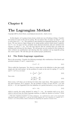
VI-2CHAPTER 6. THE LAGRANGIAN METHODproblem involves more than one coordinate, as most problems do, we just have to apply eq.(6.3) to each coordinate. We will obtain as many equations as there are coordinates. Eachequation may very well involve many of the coordinates (see the example below, where bothequations involve both x and θ).At this point, you may be thinking, “That was a nice little trick, but we just got luckyin the spring problem. The procedure won’t work in a more general situation.” Well, let’ssee. How about if we consider the more general problem of a particle moving in an arbitrarypotential V (x) (we’ll stick to one dimension for now). The Lagrangian is thenL 1mẋ2 V (x),2(6.5)and the Euler-Lagrange equation, eq. (6.3), givesmẍ dV.dx(6.6)But dV /dx is the force on the particle. So we see that eqs. (6.1) and (6.3) togethersay exactly the same thing that F ma says, when using a Cartesian coordinate in onedimension (but this result is in fact quite general, as we’ll see in Section 6.4). Note thatshifting the potential by a given constant has no effect on the equation of motion, becauseeq. (6.3) involves only the derivative of V . This is equivalent to saying that only differencesin energy are relevant, and not the actual values, as we well know.In a three-dimensional setup written in terms of Cartesian coordinates, the potentialtakes the form V (x, y, z), so the Lagrangian isL 1m(ẋ2 ẏ 2 ż 2 ) V (x, y, z).2(6.7)It then immediately follows that the three Euler-Lagrange equations (obtained by applyingeq. (6.3) to x, y, and z) may be combined into the vector statement,mẍ V.(6.8)But V F, so we again arrive at Newton’s second law, F ma, now in three dimensions.Let’s now do one more example to convince you that there’s really something nontrivialgoing on here.θl xmFigure 6.1Example (Spring pendulum): Consider a pendulum made of a spring with a mass m onthe end (see Fig. 6.1). The spring is arranged to lie in a straight line (which we can arrangeby, say, wrapping the spring around a rigid massless rod). The equilibrium length of thespring is . Let the spring have length x(t), and let its angle with the vertical be θ(t).Assuming that the motion takes place in a vertical plane, find the equations of motion for xand θ.Solution: The kinetic energy may be broken up into the radial and tangential parts, so wehave³ 1T m ẋ2 ( x)2 θ̇2 .(6.9)2The potential energy comes from both gravity and the spring, so we haveV (x, θ) mg( x) cos θ The Lagrangian is thereforeL T V ³1 2kx .2(6.10) 11m ẋ2 ( x)2 θ̇2 mg( x) cos θ kx2 .22(6.11)

6.1. THE EULER-LAGRANGE EQUATIONSVI-3There are two variables here, x and θ. As mentioned above, the nice thing about the Lagrangian method is that we can just use eq. (6.3) twice, once with x and once with θ. So thetwo Euler-Lagrange equations areddt³ L ẋ L x mẍ m( x)θ̇2 mg cos θ kx,(6.12)andddt³ L θ̇ L θ d ¡m( x)2 θ̇ mg( x) sin θdt m( x)2 θ̈ 2m( x)ẋθ̇ mg( x) sin θ. m( x)θ̈ 2mẋθ̇ mg sin θ.(6.13)Eq. (6.12) is simply the radial F ma equation, complete with the centripetal acceleration, ( x)θ̇2 . And the first line of eq. (6.13) is the statement that the torque equals the rateof change of the angular momentum (this is one of the subjects of Chapter 8). Alternatively,if you want to work in a rotating reference frame, then eq. (6.12) is the radial F maequation, complete with the centrifugal force, m( x)θ̇2 . And the third line of eq. (6.13) isthe tangential F ma equation, complete with the Coriolis force, 2mẋθ̇. But never mindabout this now. We’ll deal with rotating frames in Chapter 10.2Remark: After writing down the E-L equations, it is always best to double-check them by tryingto identify them as F ma and/or τ dL/dt equations (once we learn about that). Sometimes,however, this identification isn’t obvious. And for the times when everything is clear (that is, whenyou look at the E-L equations and say, “Oh, of course!”), it is usually clear only after you’ve derivedthe equations. In general, the safest method for solving a problem is to use the Lagrangian methodand then double-check things with F ma and/or τ dL/dt if you can. At this point it seems to be personal preference, and all academic, whether you use theLagrangian method or the F ma method. The two methods produce the same equations.However, in problems involving more than one variable, it usually turns out to be mucheasier to write down T and V , as opposed to writing down all the forces. This is becauseT and V are nice and simple scalars. The forces, on the other hand, are vectors, and it iseasy to get confused if they point in various directions. The Lagrangian method has theadvantage that once you’ve written down L T V , you don’t have to think anymore. Allyou have to do is blindly take some derivatives.3When jumping from high in a tree,Just write down del L by del z.Take del L by z dot,Then t-dot what you’ve got,And equate the results (but quickly!)But ease of computation aside, is there any fundamental difference between the two methods? Is there any deep reasoning behind eq. (6.3)? Indeed, there is. . .2 Throughout this chapter, I’ll occasionally point out torques, angular momenta, centrifugal forces, andother such things when they pop up in equations of motion, even though we haven’t covered them yet. Ifigure it can’t hurt to bring your attention to them. But rest assured, a familiarity with these topics is byno means necessary for an understanding of what we’ll be doing in this chapter, so just ignore the referencesif you want. One of the great things about the Lagrangian method is that even if you’ve never heard of theterms “torque,” “centrifugal,” “Coriolis,” or even “F ma” itself, you can still get the correct equationsby simply writing down the kinetic and potential energies, and then taking a few derivatives.3 Well, you eventually have to solve the resulting equations of motion, but you have to do that with theF ma method, too.

VI-46.2CHAPTER 6. THE LAGRANGIAN METHODThe principle of stationary actionConsider the quantity,Zt2L(x, ẋ, t) dt.S (6.14)t1y1t-g/2Figure 6.2S is called the action. It is a quantity with the dimensions of (Energy) (Time). S dependson L, and L in turn depends on the function x(t) via eq. (6.1).4 Given any function x(t),we can produce the quantity S. We’ll just deal with one coordinate, x, for now.Integrals like the one in eq. (6.14) are called functionals, and S is sometimes denotedby S[x(t)]. It depends on the entire function x(t), and not on just one input number, as aregular function f (t) does. S can be thought of as a function of an infinite number of values,namely all the x(t) for t ranging from t1 to t2 . If you don’t like infinities, you can imaginebreaking up the time interval into, say, a million pieces, and then replacing the integral bya discrete sum.Let’s now pose the following question: Consider a function x(t), for t1 t t2 , whichhas its endpoints fixed (that is, x(t1 ) x1 and x(t2 ) x2 , where x1 and x2 are given),but is otherwise arbitrary. What function x(t) yields a stationary value of S? A stationaryvalue is a local minimum, maximum, or saddle point.5For example, consider a ball dropped from rest, and consider the function y(t) for 0 t 1. Assume that we somehow know that y(0) 0 and y(1) g/2. 6 A number ofpossibilities for y(t) are shown in Fig. 6.2, and each of these can (in theory) be plugged intoeqs. (6.1) and (6.14) to generate S. Which one yields a stationary value of S? The followingtheorem gives us the answer.Theorem 6.1 If the function x0 (t) yields a stationary value (that is, a local minimum,maximum, or saddle point) of S, thenµ¶d L L .(6.15)dt ẋ0 x0It is understood that we are considering the class of functions whose endpoints are fixed.That is, x(t1 ) x1 and x(t2 ) x2 .Proof: We will use the fact that if a certain function x0 (t) yields a stationary value of S,then any other function very close to x0 (t) (with the same endpoint values) yields essentiallythe same S, up to first order in any deviations. This is actually the definition of a stationaryvalue. The analogy with regular functions is that if f (b) is a stationary value of f , thenf (b ²) differs from f (b) only at second order in the small quantity ². This is true becausef 0 (b) 0, so there is no first-order term in the Taylor series expansion around b.Assume that the function x0 (t) yields a stationary value of S, and consider the functionxa (t) x0 (t) aβ(t),(6.16)where a is a number, and where β(t) satisfies β(t1 ) β(t2 ) 0 (to keep the endpointsof the function fixed), but is otherwise arbitrary. When producing the action S[xa (t)] in(6.14), the t is integrated out, so S is just a number. It depends on a, in addition to t1 and4 In some situations, the kinetic and potential energies in L T V may explicitly depend on time, sowe have included the “t” in eq. (6.14).5 A saddle point is a point where there are no first-order changes in S, and where some of the second-orderchanges are positive and some are negative (like the middle of a saddle, of course).6 This follows from y gt2 /2, but pretend that we don’t know this formula.