Transcription
IntroductiontoCurves and SurfacesSIGGRAPH 1996Dr. Alyn P. RockwoodOrganizerPeter ChambersAuthor & PresenterDr. Hans HagenPresenterThomas McInerneyPresenterCopyright 1996, Alyn Rockwood and Peter Chambers1
AbstractThis course presents an introduction to CAGD—Computer-Aided GeometricDesign. The mathematical tools required to create well-behaved curves andsurfaces are covered, together with efficient algorithms for their implementation.Topics covered include basis functions, Bézier curves, B-splines, and surfacepatches.2
Table of ContentsTopicPageIntroduction to CAGD10Preliminary Mathematics18The Bézier Curve32Blossoms53The B-Spline Curve64Surfaces76Bibliography873
Course ContributorsDr. Alyn P. RockwoodAlyn P. Rockwood completed B.S. and M.S. degrees in mathematics at BrighamYoung University and a Ph.D. at the Dept. of Applied Mathematics andTheoretical Physics of Cambridge University, Cambridge, England. He worked inindustrial research for 13 years, including supervisory and research positions atEvans and Sutherland Computer Corp. and Silicon Graphics, Inc. He wasinvolved in flight simulation, CAD/CAM and surface rendering projects at thesecompanies.Currently, he is on the computer science faculty at Arizona State University. Hisinterests include computer graphics, scientific visualization and computer aidedgeometric design. He has several patents and many publications in these fields.Peter ChambersPeter Chambers received his B.Sc. from the University of Exeter, England, andhis M.S. from Arizona State University. Peter is an Engineering Fellow in theAdvanced Multimedia Group at VLSI Technology, Tempe, Arizona. His areas ofinterest at VLSI include circuit design, computer architectures, and peripheralinterfaces for personal computers.Peter has architected and designed numerous products, including theInput/Output systems for minicomputers, and many large integrated circuits.Peter's other interests include high level hardware description languages,techniques for robust design, and interface performance analysis.Peter's involvement with Arizona State University includes research on texturingmethods in computer graphics and interactive learning tools. His most recentpublication is Interactive Curves and Surfaces, in collaboration with AlynRockwood, upon which these course notes are based.4
Dr. Hans HagenHans Hagen is a professor of computer science at the University ofKaiserslautern, Germany. His research centers on geometric modeling andscientific visualization.Dr. Hagen received his B.A. and his M.S. from the University of Freiburg and hisPh.D. from the University of Dortmund. Before moving to Kaiserslautern he heldfaculty positions at the University of Braunschweig and at Arizona StateUniversity. He is one of the current directors at the Dagstuhl Conference andResearch Center.Dr. Hagen is on the editorial board of Computer Aided Geometric Design,Transactions on Visualization and Computer Graphics, Computer Aided Design,Computing, and Surveys on Mathematics for Industry.Thomas McInerneyThomas McInerney writes code for Apple Computer during his summers. Hisinterests are in computer graphics and computer networks. He is completing hisB.S. in Computer Science from Arizona State University. He is also writing theJava version of the curves and surfaces book with Alyn Rockwood andPeter Chambers.5
Interactive Curves and Surfaces:A Multimedia Tutorial on CAGDAlyn RockwoodArizona State UniversityPeter ChambersVLSI Technology, Inc.Now available this book/disk package is an interactive multimedia software tutorialon computer-aided geometric design that runs under Windows 3.1 and Windows 95.This innovative tutorial allows you to: Learn and understand the uses of computer-aided geometric design (CAGD) inscience and industry. Become familiar with standard ways of creating curved lines and surfaces,including Bézier curves, B-Splines, and parametric surface patches. Understand the mathematical tools behind the generation of these objects, andthe development of computer-based CAGD Algorithms. Use powerful interactive test benches to explore the behavior and characteristicsof the most popular CAGD curves.CONTENTS:Introductionto CAGDPreliminary MathematicsThe Bézier CurveInterpolationBlossomsThe B-Spline CurveRational CurvesSurfacesTwo 3.5" diskettes with accompanying paperback bookISBN 1-55860-405-7 / Price: 59.9525% DISCOUNT COUPONPresent this coupon to Morgan Kaufmann Publishers at Booth #1611and receive a 25% discount on your copyInteractive Curves and Surfaces:A Multimedia Tutorial on CAGDby Alyn Rockwood and Peter ChambersTwo 3.5" diskettes with accompanying paperback bookISBN 1-55860-405-7 / Price: 59.95Discount offer valid only at SIGGRAPH 1996 Marketing / Code CSGR6
Contact InformationAlyn RockwoodDr. Alyn P. RockwoodDepartment of Computer ScienceArizona State UniversityTempeArizona 85287Phone:602 965 8267email:rockwood@asu.eduPeter ChambersPeter ChambersVLSI Technology8375 South River ParkwayTempeArizona 85284VLSI T ECHNOLOGYPhone:602 752 6395email:peter.chambers@vlsi.comHans HagenProf. Dr. Hans HagenUniversity of KaiserslauternFB Informatik / AG Hagen 36/226Postfach 304967663 KaiserslauternGermanyPhone:49 631 205 4071email:hagen@informatik.uni-kl.de7
Thomas G. McInerneyThomas G. McInerney2929 N. 70th St. # 2089ScottsdaleArizona 85251Phone:602 970 7643email:tgm@asu.edu8
AcknowledgmentsAlyn Rockwood and Peter Chambers wish to thank:Mike Morgan and Marilyn Uffner Alan at Morgan Kaufman, for making theInteractive Curves and Surfaces project possible.Spencer Thomas, Jim Miller, Aristides Requicha, and Jules Bloomenthal, fortheir excellent comments and ideas.Shara-Dawn Simon, for her diligent proof-reading, and the significantimprovements in layout and flow she suggested.Professor Don Evans, director of the Center of Innovation in EngineeringEducation, of the College of Engineering and Applied Science, Arizona StateUniversity, for support and encouragement.The authors also appreciate the sponsorship of the US/Hungarian Science andTechnology Joint Fund, in cooperation with Arizona State University, project396.9
Topic 1Introduction toCAGD10
Topic 1: Introduction to CAGDIn this topic, you will: Learn what CAGD is about. Learn some of the history of CAGD. See some typical applications of CAGD tools.What CAGD is All AboutComputer-Aided Geometric Design is a new field that initially developed tobring the advantages of computers to industries such as: Automotive Aerospace ShipbuildingCAGD expanded rapidly and now pervades many areas, from pharmaceuticaldesign to animation. We are surrounded by products that are first visualizedon a computer. These products are modified and refined entirely within thecomputer; when the product enters production, the tools and dies areproduced directly from the geometry stored in the computer. This process isknown as virtual prototyping.(c) 1995 Autodesk, Inc. This image was provided courtesy of Autodesk, Inc.11
Computer visualizations of new products reduce the design cycle by easingthe process of design modification and tool production.CAGD is based on the creation of curves and surfaces, and is accuratelydescribed as curve and surface modeling. Using CAGD tools with elaborateuser interfaces, designers create and refine their ideas to produce complexresults. They combine large numbers of curve and surface segments to realizetheir ideas. However, the individual segments they use are relatively simple,and it is at this level that the study of CAGD is concentrated.A Design Challenge: The Need for CAGDWhen creating products and artwork, designers face tasks such as this:You are given two points in a plane and two directions associated with thepoints. Find the curve that passes through the points that is tangent to the givendirections:This is a simple task for anyone with a pencil and paper who is familiar withparametric forms, the types of curves used in CAGD.CAGD produces tools are meant to be: Intuitive Simple to useSometimes the mathematics underlying the tools becomes quite sophisticated,yet the result is meant to be easily understood and geometrically intuitive.12
The technical person often benefits from these intuitive and visually related toolswhen considering deeper mathematical problems. The geometry of CAGD isvery amenable to visual demonstration.CAGD: From Points to TeapotsThere is a natural progression of the geometry behind CAGD. With smallincremental steps it is possible to describe complex objects in terms of simpleprimitives, such as points and lines. Control Points: The Start of CAGDTake four points in a plane and connecting them to form a polygon. The pointsare known as Control Points 1, and the polygon as the Control Polygon 2. Thecontrol points and polygon determine the approximate shape of the curve to beformed.1Control points are points in two or more dimensions which define the behaviorof the resulting curve.2The control polygon is formed by connecting the control points in the correctorder. The control polygon provides a crude analogy of the refined curve. Notethat the control polygon is typically open (the ends are not coincident), and itmay self-intersect arbitrarily.13
A CAGD Favorite: The Bézier CurveA special curve known as the Bézier Curve 3 may be generated by the controlpoints. Note that while the curve passes through the end points, it only comesclose to the other points. Three-Dimensional Control Polygons for Surfaces (Control Meshes)Bézier curves behave just as well in three dimensions as in two. This figureshows the control polygons for a three-dimensional object consisting of Bézierpatches4.3The Bézier curve, named after the French researcher Pierre Bézier, is asimple and useful CAGD curve. It is a very well behaved curve with usefulproperties, as you will discover in Topic 3, The Bézier Curve.4 A Bézier patch is a three-dimensional extension of a Bézier curve. It is formedby extruding a Bézier curve through space to form a surface.14
Three-Dimensional Wireframe ModelWhen the Bézier curves are created and connected in three dimensions, awireframe model of the object is produced. Three-Dimensional Shaded ObjectIf the surface produced by the three-dimensional Bézier patches is illuminatedand shaded, an object with a realistic appearance results. The Utah teapot, ondisplay at the Boston Museum of Computer History, is a classic in CAGD andcomputer graphics.15
The History of CAGDComputer Aided Geometric Design has mathematical roots that stretch back toEuclid and Descartes. Its practical application began with automatedmachinery to compute, draft, and manufacture objects with freeform surfaces.Production pressures in the aircraft industry during World War II stimulatedmany new devices to enhance and accelerate design and manufacturing. Forexample, in 1944 Liming designed fuselage spars with a "super-elliptic"method that could be implemented with an electro-mechanical calculator.Shipbuilders also became interested in CAGD early on. One example of theirmotivation may sound whimsical but was a serious impediment to ship design.The only place large enough to draw full scale plans for a ship was in the loftof the shipbuilders dry-dock. The huge drawings would warp and shrink in themoist air, causing very real manufacturing problems.Computers provided the greatest stimulus because of their power to enablenew ideas. In 1963, Ferguson developed one of the first surface patch systemsby which individual curvilinear patches are joined smoothly to create thesurface "quilt." He also introduced the notion of parametrically definedsurfaces which has become the standard because it provides freedom from anarbitrarily fixed coordinate system. Vertical tangent vectors can be defined bydifferentiation, for instance, which is not possible in explicit Cartesian form.In the mid 1960's automotive companies became involved in CAGD, as a wayto drive milling machines. Car bodies were designed by artists using claymodels. Painstaking measurements produced data that could drive numericallycontrolled milling machines to produce stamp molds. The initial use of CAGDwas to represent the data as a smooth surface for numerical control. It soonbecame apparent that the surfaces could be used for the design.In 1971, Pierre Bézier reformulated Ferguson's ideas so that a draftsmanwithout any extensive mathematical training could design a surface. Bezier'ssystem, UNISURF, was used by Renault and became a milestone in thedevelopment of CAGD. It epitomized the difference between surface fitting andsurface design. The purpose of design was to provide the draftsman, who hadstrong intuition about shape but limited mathematical training, computer toolsthat empowered him or her to use the sophisticated mathematics of surfacerepresentation.In the meantime, the mathematical underpinnings of CAGD continued toadvance. de Casteljau examined triangular patches and developed evaluationtechniques. Coons [Coons64] unified much of the previous work into a generalscheme which became the basis of the early modeler PDGS made by Ford. AtGeneral Motors in 1974, Gordon and Riesenfeld exploited the properties of Bspline curves and surfaces for design.Driven primarily by the automotive, shipbuilding and aerospace industries,both the mathematics of CAGD and the designer interface tools continued to16
improve through the 1970's. The first CAGD conference was organized byBarnhill and Riesenfeld in 1974, where the term "CAGD" was first used[Barnhill74].In the 1980's, the power and versatility of computer-aided designing seemedsuddenly to be discovered by anyone who had a freeform geometric surfaceapplication. Industrial designers were smitten with the power of computerdesign, and many commercial modelers become the basis of severalsubstantial applications, including: CATIA, EUCLID, STRIM, ANVIL, andGEOMOD. Geoscience used CAGD methods to represent seismic horizons;computer graphics designers modeled their objects with surfaces, as didmolecule designers for pharmaceuticals. Architects discovered them, wordprocessing and drafting programs based their interface protocols on freeformcurves (PostScript 5), and even moviemakers discovered the power ofanimating with such surfaces, beginning with TRON, continuing throughJurassic Park6, and beyond.What has Been Accomplished in this TopicThe ideas and principles behind CAGD have been introduced, together with theclassic example of surface patch use, the Utah teapot. The short but significanthistory of CAGD has been summarized.5PostScript is a proprietary page-description language used by typesetters todefine elements of printed text, including letter outlines, text layout, andgraphical images.6Jurassic Park made extensive use of CAGD and computer graphics tovisualize animated objects.17
Topic 2PreliminaryMathematics18
Topic 2: Preliminary MathematicsIn this topic, you will learn: The basic math needed for the rest of the book. An overview of parametric forms: a convenient way of describing curvesand surfaces. An illustration of linear interpolation, one of the most fundamentalconcepts in CAGD. The idea of continuity, to ensure that curves and surfaces join togethersmoothly.The Mathematics of CAGDCAGD treats points, lines, and surfaces as mathematical objects, describedgeometrically in two- or three-dimensional space.This book develops the mathematics in a step-by-step fashion, and does notdemand a rigorous mathematical background. It is recommended that thereader be familiar with the following topics: Geometry of points, lines, and planes. Equations in parametric form. Basic calculus.19
Parametric FormsCAGD relies on parametric forms to describe curves and surfaces. Manystudents of CAGD do not initially appreciate the subtlety and importance ofthis form. If you are confident with parametric forms then you may skip thissection.The Parametric CurveTypically, when a student takes mathematics, a curve is presented as agraph of a function f(x).y f(x)Graph of the setof points (x, y)xAs x is varied, y f(x) is computed by the function f, and the pair ofcoordinates (x, y) sweeps out the curve. This is called the explicit form of thecurve.20
From a design standpoint the explicit form is deficient in several ways: Single-Valuedy f(x)The circle has twovalues along this linexThe curve is single-valued along any line parallel to the y axis. For example,only parts of the circle may be defined explicitly. Infinite Slopey f(x)The circle has twopoints with infinite slopexAn explicit curve cannot have infinite slope; the derivative f' (x) is not definedparallel to the y axis. Hence there are two points on the circle that cannot bedefined. Transformation ProblemsAny transformation, such as rotation or shear, may cause an explicit curve toviolate the two points above.21
The parametric form of a curve is not subject to these limitations. Moreover, itprovides a method, known as parameterization 1, that defines motion on thecurve. Motion on the curve refers to the way that the point (x, y) traces outthe curve.Defining the Parametric CurveA parametric curve that lies in a plane is defined by two functions, x(t) andy(t), which use the independent parameter t. x(t) and y(t) are coordinatefunctions, since their values represent the coordinates of points on the curve.As t varies, the coordinates (x(t), y(t)) sweep out the curve. As an exampleconsider the two functions:x(t) sin(t), y(t) cos(t).(2.1)As t varies from zero to 2π, a circle is swept out by (x(t), y(t)). The Parametric Circle: t 0.16 (approximately 57 degr ees)1Parameterization uses an independent parameter or variable to computepoints on the curve. It gives the "motion" of a point on the curve.22
CAGD deals primarily with polynomial 2 or rational functions 3, nottrigonometric functions as shown in the examples above. For example, thecircle can also be given by allowing t to vary from -infinity to infinity in thefollowing functions:(())1 t22t, y(t) .x(t) 1 t21 t2()(2.2)As an exercise, verify for yourself that the functions in equation 2.2 doindeed generate a circle. Plot points (x(t), y(t)) or write a program to do thisfor you.Both equation 2.1 and equation 2.2 yield circles, so how do they differ? It isthe parameterization. The motion of the point (x(t), y(t)) is different, even ifthe paths (the circles) are the same.A good physical model for parametric curves is that of a moving particle 4.The parameter t represents time. At any time t the position of the particle is(x(t), y(t)). Two paths (curves) may be identical even though the motion(parameterization) is different.Parametric curves are not constrained to be single-valued along any line(recall the single-valued deficiency of the explicit form), and the slope of aparametric curve segment may be defined vertically. The slope is given bythe tangent line at any point, computed by finding the derivative vector (x'(t),y'(t)) at any point t. This vector determines the speed at which the pointtraces out the curve as t changes.Curves defined by points whose speed may drop to zero do cause problemsthat will be considered later under the discussion of continuity.2A polynomial is a function of the form:p(t) a 0 a1t a 2 t 2 . a n t n , where the a i are scalars or vectors.3A rational function is made by dividing one polynomial by another, forexample:1 2t 3t 3 t 4r(t) .1 2t 2A rational function may contain vector coefficients only within the numerator.4As the parameter t changes, the coordinate point (x(t), y(t)) traces the curve.This point can be thought of as a particle that moves under the influence ofchanges in the value of the parameter t.23
Consider the parametric curve given by these two coordinate functions:x(t) 6t 9t 2 4t3,y(t) 4t 3 3t 2. (2.3)Bézier tangent demonstrationThe illustration above demonstrates the following for this parametric curve,as t varies between 0 and 1: The parameter t moves the point (x(t), y(t)) along the path of the curve. The point's speed varies as t varies. The speed is higher at the ends ofthe curve. The derivative vector changes in length, reflecting the variation in thespeed of the point. In the demonstration, the curve crosses itself, which can easily happenwith parametric curves.A convenient notation for equation 2.3 is:24
x(t ) 6 9 4 f(t) t t 2 t 3. 3 4 y(t) 0 (2.4)Equations 2.3 and 2.4 are the same. We simply save on notation by writingthe basis functions 5 only once, which are then multiplied by the appropriatevectors. When a vector is multiplied by a scalar, each coordinate in thevector is individually multiplied by the scalar.In general, a parametric polynomial is written as:f(t) a0 a1t a 2 t 2 . an t n .(2.5)where f(t) is a vector-valued function, and the a's are vectors. The vectorsare not restricted to two dimensions. The a's might be vectors of threedimensions, for instance. In this case the function f(t) would have threecoordinate functions x(t), y(t), and z(t). The curve would be a curve in space,and the derivative f'(t) would be given by the vector of the derivativecoordinate functions (x'(t), y'(t), z'(t)).The general case described by equation 2.5 includes a constant term ( a0),which the example given by equations 2.3 and 2.4 does not have.Here, the basis functions are 1, t, t 2 , and t 3 . 0 The coefficient for the basis function "1" is . 0 525
The Parametric SurfaceAs with curves, it is typical for the reader to have encountered surfacesexplicitly as z f(x, y). Often called elevation surfaces or terrain, the height zis given at a point on the plane by computing f(x, y). Such a surface definitionshares the same flaws mentioned previously for curves: They must be single-valued for any point on the plane. They cannot have vertical tangent planes. Transformations may cause the above two difficulties.The parametric form of the surface corrects these problems. In order todefine a parametric surface, it is best to first define a parametric curve, andthen sweep the curve through space to define the surface.Consider a planar curve given by:x(t ) 2 2 t,(2.6)y(t ) 2 t 2 t 2.Or in vector form, x(t ) 2 2 0 t t 2. 2 y(t ) 0 2 (2.7)The curve given by x(t) and y(t) looks like this:yx(t) 2 - 2ty(t) 2t-2t 2(x(t), y(t))0.5x002Here, the parameter t is limited to the range 0 to 1.The curve becomes a surface in three dimensions if another parameter s andanother coordinate function z are added. Consider, for instance:26
x(s, t ) 2 2 t,y(s, t ) 2 t 2 t 2,(2.8)z(s, t ) s.When s 1, the curve defined by equation 2.5 is produced on the planez 1. As this curve changes in s it sweeps out a surface. A parametricsurface may be thought of as a bundle of parametric curves; by fixing s or ton a surface, one single curve from this bundle is selected.In this figure, the planar curve is extruded through the z dimension tobecome a surface. When s 0.8, the curve is produced as t varies between0 and 1.In equation 2.8, x(s,t) and y(s,t) have no terms in s, and z(s,t) has no term int. The terms are limited to simplify the example, but this is not typical. Ingeneral the surface may be written as the parametric polynomial: x(s, t) f(s, t) y(s, t) z s, t ( ) (2.9) a00 a10 s a01 t a11 s t a20 s2 a02 t 2 a21 s2 t .Bold letters indicate vector quantities. The indices of the a-vectorscorrespond to the parametric powers.27
ContinuityThe notion of continuity 6 was developed for explicit functions to describewhen a curve does not break or tear. If it meets these conditions, it isdescribed as C 0. C0 continuity is defined by the popular description: "A curveis continuous if it can be drawn without lifting the pencil from the paper."If the derivative curve is also continuous, then the curve is first-orderdifferentiable and is said to be C 1 continuous. Extending this idea, it is saidthat a curve is Ck differentiable if the kth derivative curve is continuous.Practically, this means that a C 1 continuous curve will not kink. Higherdegrees of continuity imply a smoother curve.A C 0 CurveA C 1 CurveTwo curves are shown here, one that is C 0 and one that is C 1. The C 0 curvehas a kink, while the C 1 curve is generally smooth.The traditional notion of C 1 continuity does not, in fact, ensure much aboutthe curve's properties. Imagine, for instance, a particle that travels in astraight line but has distinct jumps in velocity. It is not C 1, but the curve iscertainly smooth. Conversely, it is possible to have a C 1 curve with a kink init. This can occur when the velocity of the particle goes to zero where itchanges direction and starts up again. This is illustrated in the followingfigure:6Continuity implies a notion of smoothness, that is, curves which are notjagged or which break. Commercial applications of CAGD, for example carbody design, frequently require that curves and surfaces are continuous.28
Mathematicians have developed the concept of a manifold as a new way ofdescribing continuity. In CAGD there is a simpler concept to achieve thesame end. It is the idea of geometric continuity 7. If a curve is C 0, it is G 0continuous. If a curve's tangent direction changes continuously then it is G 1continuous. Its magnitude may jump discontinuously but the curve is still G 1.Hence a particle traveling at erratically changing speeds may still trace out asmooth curve if its direction changes smoothly. This is illustrated in thefollowing figure:Sudden changein tangent lengthIf a C1 curve has kinks because its derivative goes to zero at a point, thenthis curve will not be G 1, since the tangent direction changes discontinuouslyat the kink. Hence the notion of geometric continuity provides a useful way tounderstand the smoothness of a curve or surface.7Geometric continuity introduces a notation that immediately tells the designerwhether or not the curve is smooth.29
Linear InterpolationGiven two points in space, a line can be defined that passes through themboth in parametric form:l(t ) (1 t )b0 t b1,(2.11) x x where b0 0 and b1 1 , the two points in space. y0 y1 Thus l(t) is a point somewhere in space, depending on the parameter t. Linear interpolation between two points: t 0.125.The screen captured from the interactive demonstration displays only twoplaces after the decimal point.Linear interpolation is perhaps the most fundamental concept. Allsubsequent curves and surfaces are defined by repeated linear interpolationin some form.Other forms of linear interpolation are possible. For example,30
l(t ) t b0 t 1 b1,10 10 which also gives a straight line through the two points. Note that:l(0) b1 and l(10) b0.This is the same straight line (a linear combination of the two points), but ithas a different parameterization. That is, the motion of a particle at t isdifferent. In most cases it is preferable to start at t 0 and end at t 1.What has Been Accomplished in this TopicThe background to parameterized curves and surfaces has been covered inconsiderable detail. The hodograph visualized the behavior of the derivative ofa curve, and clarified the concept of the motion of a point on the curve.Continuity was introduced to manage the boundaries between multiple curvesor surfaces, and extended to include geometric continuity. Finally, linearinterpolation was considered as a prerequisite for Bézier curves andblossoming.31
Topic 3The Bézier Curve32
Topic 3: The Bézier CurveIn this topic, you will learn: What a Bézier curve is. The properties and behavior of the Bézier curve. How to create a Bézier curve. The de Casteljau algorithm for evaluati on of a Bézier curve. Subdivision and differentiation of the Bézier curve.Introduction to the Bézier CurveThe Bézier curve is a good place to start a study of CAGD. It underpins otherconcepts such as B-splines and surface patches. It is visually engaging andexhibits many desirable properties for design. The cubic Bézier curve:33
Mathematical Properties of the Bézier CurveConsider the parabola that passes through (0,1) and (1,0) and is tangent to the xand y axes at these points:0,11,0The parametric form of a parabola looks like:f(t ) a t 2 b t c,(3.1)where a, b, and c are vector coefficients. f(t) is a vector function which has twocomponents, i.e. f(t) (x(t), y(t)). The above parabola can be written as 1 2 1 f(t) t 2 t . 1 0 0 (3.2)This can be rewritten as: 1 0 0 2f(t) (1 t) 2t(1 t) t 2 . 0 0 1 (3.3)The reformation process is shown below 1.1This parabola is defined parametrically by:y(t ) t 2and:x(t ) 1 2 t t 2 (1 t ) .234
This is exactly the same curve as equation 3.2, so what advantage is there inrewriting? The advantage lies in the geometrical meaning of the coefficients:(1,0), (0,0), and (0,1). These are called control points. Together, the controlpoints form the control polygon.Observe: The curve passes through the endpoints of the control polygon. The curve is cotangent to the control polygon at these endpoints.The curve in this form is called the Bézier curve, and the observations hold ingeneral for any coefficients. This means that if the coefficients are changed, thecurve changes in an easy-to-understand way. The quadratic Bézier curve:In vector form, it may be expressed as: x(t) 1 0 0 22f(t) (1 t) 2 t (1 t) t . 0 1 y(t) 0 35
The general form for a quadratic Bézier curve is:f(t ) b0 (1 t ) b1 2 t (1 t ) b2 t 2 .2(3.4)This is a parabola exactly as equation 3.1 but it is rewritten so that the controlpointsb0, b1, and b2 have geometrical significance as the control points of theparabola.Bézier Curves of General DegreeThe general form of a Bézier curv
on computer-aided geometric design that runs under Windows 3.1 and Windows 95. This innovative tutorial allows you to: Learn and understand the uses of computer-aided geometric design (CAGD) in science and industry. Become familiar