Transcription
IEEE Power & Energy SocietyJan 2013TECHNICAL REPORTPES-TR1Dynamic Models forTurbine-Governors inPower System StudiesPREPARED BY THEPower System Dynamic Performance CommitteePower System Stability SubcommitteeTask Force on Turbine-Governor Modeling IEEE 2013 The Institute of Electrical and Electronic Engineers, Inc.No part of this publication may be reproduced in any form, in an electronic retrieval system or otherwise, without the prior written permission of the publisher.
THIS PAGE LEFT BLANK INTENTIONALLYii
TASK FORCE ONTURBINE-GOVERNOR MODELINGCHAIRMAN: POUYAN POURBEIKMEMBERS AND CONTRIBUTORSRoy BoyerKevin ChanGraeme ChownJames FeltesCarlos Grande-MoranLuc Gérin-LajoieFritz LangenbacherDaniel LeonardLeonardo LimaLes HajagosLouis HannettWolfgang HofbauerFhedzi ModauMahendra PatelShawn PattersonStefan SterpuAlex SchneiderJohn Undrilliii
ACKNOWLEDGEMENTSThe Task Force (TF) is part of the IEEE Power & Energy Society, reporting through thePower System Stability Subcommittee of the Power System Dynamic PerformanceCommittee. The Scope was approved in June 2007 by the Power System StabilitySubcommittee and by the Power System Dynamic Performance Committee. We are trulygrateful for the support of our sponsoring subcommittee and committee.The Task Force gratefully acknowledges the participation of the following individuals inthe TF meetings (or by email) and their feedback, comments and suggestions: Eric Allen,Elmer Bourque, Bob Cummings, Donald Davies, Michael Gibbard, Sven Granfors,Joseph Hurley, Howard Illian, Dmitry Kosterev, Juan J. Sanchez-Gasca, Lee Taylor,Chavdar Ivanov, David Vowles and Anthony Williamsiv
CONTENTSContents1. INTRODUCTION . 1-11.1The Scope of Work . 1-11.2The Purpose of Turbine-Governor Models in Power System Studies . 1-12. STEAM TURBINES . 2-12.1Steam Turbine Modeling . 2-12.2Simple Steam Turbine Models (TGOV1, IEEESO and IEEEG1) . 2-12.3Simple Steam Turbine Model with Basic Boiler Dynamics [13] . 2-42.4Detailed Steam Turbine Model – the TGOV5 model . 2-92.4.1 The TGOV5 model. 2-92.4.2An Example use of the TGOV5 Model . 2-102.4.2.1 Primary Frequency Control Deadband and Limiter . 2-122.5Simulating Fast-Valving . 2-142.6Other Aspects of Steam Turbine Modeling . 2-142.7Modeling Guidelines and Summary . 2-173. GAS TURBINES AND COMBINED CYCLE POWER PLANTS . 3-13.1Gas Turbine Modeling . 3-13.1.1Brief Overview of Gas Turbine Theory . 3-13.1.2Modeling Gas Turbines . 3-33.1.2.1 GAST. 3-33.1.2.2 GAST2A. 3-43.1.2.3 GGOV1. 3-43.1.2.4 CIGRE model [9] . 3-83.1.2.5 Simplified but Explicit Modeling of the Ambient and Speed Dependence [16]3-103.1.2.6 Vendor Specific Models . 3-133.2Combined Cycle Power Plants . 3-133.2.1Brief Overview of CCPP . 3-133.2.2Implementation of the CIGRE HRSG and ST model in ERCOT . 3-143.3Modeling Guidelines and Summary . 3-194. Hydro Turbines . 4-14.1Modeling Hydro Turbines . 4-14.2Hydro Governors . 4-24.3Hydro Water Column . 4-54.4System Frequency Regulation Studies . 4-94.5Modeling Guidelines and Summary . 4-115. References. 5-16. Further Reading on Turbine-Governor Modeling . 6-1APPENDIX A: Parameters for the IEEEG1 LCBF1 Model . A-1APPENDIX B: Deadband . B-1APPENDIX C: Typical Parameters for the GGOV1 . C-1APPENDIX D: Vendor Specific Model for GE Heavy-Duty Gas Turbines. D-1APPENDIX E: Vendor Specific Model for the ALSTOM GT26B Heavy-Duty Gas Turbine . E-1APPENDIX F: ALSTOM Combined Cycle Power Plant Models . F-1APPENDIX G: Solar Turbine’s Perspective on the GT Models . G-1v
INDEX OF AUTHORSAuthors Listed in Alphabetical OrderChapter 1 IntroductionP. PourbeikChapter 2 Steam TurbinesG. Chown, J. Feltes, F. Modau, P. Pourbeik (lead-editor) and S. SterpuChapter 3 Gas Turbines and Combined Cycle Power PlantsR. Boyer, K. Chan, J. Feltes, L. Hannett, D. Leonard, L. Lima, F. Modau andP. Pourbeik (lead-editor)Chapter 4 Hydro TurbinesW. Hofbauer, L. Gérin-Lajoie, S. Patterson (lead-editor), P. Pourbeik and J.UndrillAppendix A – Parameters for the IEEEG1 LCBF1 ModelP. PourbeikAppendix B – DeadbandP. PourbeikAppendix C – Typical Parameters for the GGOV1L. Hannett and D. LeonardAppendix D – Vendor Specific Model for GE Heavy-Duty GasTurbinesL. Hannett and D. LeonardAppendix E – Vendor Specific Model for the ALSTOM GT26BHeavy-Duty Gas TurbineK. ChanAppendix F – ALSTOM Combined Cycle Power Plant ModelsK. ChanAppendix G – Solar Turbine’s Perspective on the GT ModelsF. LangenbacherMain Editor:P. Pourbeikvi
1.INTRODUCTION1.1The Scope of WorkThe scope of this Task Force is to review and make recommendations related to theuse of models for turbine‐governors for power system simulations. Recentdocuments published by CIGRE 1 , the Western Electricity Coordinating Council(WECC) and others have provided newly developed models for use in modelingthermal turbine‐governors, modern combined cycle power plants and hydroturbines. There is, however, significant benefit in reviewing the recommendations inthese documents and consolidating them with the usage of older models that stillexist in commonly used simulation programs. The Task Force report is presented inthree parts. Chapter 2 deals with steam turbines. Chapter 3 deals with gas turbinesand combined cycle power plants. Chapter 4 deals with hydro turbines. Eachdocument provides the following:1. A summary of a hierarchy of models for the various turbine‐governorsystems.2. A discussion of the various existing models in most commercial softwaretools and what may be considered as legacy models.Additionally, in this first chapter a section is provided below that discusses theprimary motive for modeling turbine‐governors and the recommended usage of themodels.In many grid‐codes around the world outside of North America, model performanceand validation requirements are defined and must be complied with as these aredeemed statutory (e.g. [1]). The Task Force has intentionally avoided the discussionof grid‐codes since such discussion are outside the scope of this group. What ispresented here is for guidance and educational purposes. This document is not astandard, nor does it claim to address or comment about any standards or grid‐codes.This Task Force was approved as a working body of the Power System StabilitySubcommittee, of the Power system Dynamic Performance Committee of the IEEEPower & Energy Society in June, 2007.1.2The Purpose of Turbine-Governor Models in Power System StudiesPower system stability studies deal primarily with transient angle and voltagestability, small‐signal stability and frequency control and stability. Reference [2]provides the definitions of each of these types of stability problems. In practice, it isnot possible to completely decouple these various stability problems from oneanother. Particularly in smaller systems, a single event could give rise to multipleinter‐related phenomena of frequency, voltage and angular stability problems.1The International Council on Large Electric Systems (www.cigre.org).1 -1
With this understanding in mind, the modeling of turbine‐governors is particularlyimportant for studies related to transient angular stability, frequency stability andcontrol, and to a lesser extent small‐signal stability.For small‐signal stability issues it is possible for the turbine‐governor to have aslight negative damping effect in the frequency range of electromechanical modes ofrotor oscillation. However, the most widely accepted means of improving thedamping of both local and inter‐area modes of rotor oscillation on synchronousgenerators is the application of power system stabilizers (PSS) [3, 4]. If the PSS isproperly tuned, it will more than compensate for any such negative dampingassociated with the turbine‐governor and the more influential source of negativedamping, high‐gain automatic voltage regulators [3].For transient rotor angle stability the turbine‐governor model is of key importance.The important aspect of the turbine‐governor dynamics is the initial response of theturbine‐governor in the initial second or two following a grid disturbance. A clearexample is the concept of fast‐valving [4]. This control is characterized by thesudden action to close the intercept valves on a steam turbine following a nearbyfault to reduce the mechanical power on the generator shaft and thus minimize theacceleration of the shaft and likelihood of rotor angle instability. Any such controlsthat will suddenly affect the mechanical output of the turbine following a nearbygrid fault would be critical to model for transient stability studies. Another exampleis the implementation of acceleration controls on gas turbines, which in some casesmay come into play during a nearby severe grid fault. Not all gas turbines haveacceleration controls. Also, where droop is implemented through feedback ofelectrical power and the use of a proportional‐integral (PI) or proportional‐integral‐derivative (PID) controller in the turbine‐governor controls (typical on manymodern gas turbines), this can have some affect on transient stability and it shouldbe modeled accordingly.The modeling of the turbine‐governor is of greatest importance when studyingfrequency control and stability. Frequency response is an important aspect ofpower system performance. Figure 1‐1a) shows a generic response of a typicalpower system to a large loss of generation. Here it is assumed that only a singleevent occurs, being the sudden and unplanned loss of major generation, due, forexample, to a failure of mechanical equipment. As can be seen in Figure 1‐1a), thereare essentially three periods of response, (i) the initial period of response down tothe nadir of the frequency deviation, which is governed by the initial rate of declineof frequency, which is a function of total system inertia and the primary‐frequencycontrol that is provided by turbine‐generator governors, (ii) the initial recovery infrequency which is determined by both primary‐frequency response (turbine‐governor control and droop) and the load behavior [5], and (iii) the final return ofthe system frequency to nominal frequency as achieved by automatic generationcontrol (AGC). A discussion of AGC is outside the scope of this Task Force. Figure 1‐1b) shows a real example of frequency response for the loss of a large generatingunit in WECC – the event is from 2008.1 -2
Clearly, when attempting to simulate such events for planning studies, the modelingand representation of turbine‐governor response on conventional generating unitsis of great importance.A detailed look at Figure 1‐1b) reveals the following facts:1. Initial rate of frequency decline 0.25Hz/s2. Minimum Frequency: 59.72 Hz reached 6 seconds after the event3. Final settling frequency before AGC action: 59.85 Hz reached 20 secondsafter the event.This is a typical trace for a large loss of generation in WECC – the event in this casewas the loss of 2.7 GW of generation. The WECC has over 300 GW of installedgeneration capacity. In comparison, for a system such as the Electric ReliabilityCouncil of Texas (ERCOT), which is roughly one‐fifth the size of WECC, frequencydips (nadir) as low as 59.6 Hz have been seen and rates of change of approximately0.2 Hz/s [6], for the loss of a large generating unit/plant in Texas. Going to an evensmaller system such as Ireland, with a large penetration of wind generation, and onecan see dips of up to 1 Hz (nadir) 2 and rates of decline of 0.5 Hz/s [7, 8]. NewZealand has reported rates of change of frequency as high as 1 Hz/s and a dip of 2.5Hz (nadir) 3 , back in 2003 [9]. With the increased penetration of wind generationthese numbers may all be larger now, and in the case of New Zealand and Irelandthey may increase significantly.It should be noted that the examples discussed above are simply examples toillustrate some concepts. The actual frequency response of these systems variesfrom event to event since the response is dependent on (i) the amount of the MWloss and (ii) the amount of MWs of responsive generation that is on‐line.With this background it is easy to appreciate that it is difficult to provide an exactspecification of model performance requirements for all possible systems and studyconditions. Furthermore, it is impractical to expect a model to be appropriate for allpossible systems and study conditions; therefore a hierarchy of models is needed.In general, however, it may be said that for typical planning studies the focus is onsimulating events for which the system remains predominantly intact (i.e. no majorislanding events). For large systems (e.g. North America) the typical deviation infrequency is at most around /‐ 1% with an initial rate of change of at most 0.3Hz/s. For smaller, island systems, the deviation may be as high as /‐ 5% with aninitial rate of change of at most 1 to 1.5 Hz/s.Validation of modes for frequency response is not a simple task, and the type ofmodel and model validation required is dependent on the time scale of interest.23For Ireland the nominal system frequency is 50 Hz so a 1 Hz dip 2 % drop in frequency.For New Zealand the nominal system frequency is 50 Hz so a 2.5 Hz dip 5% drop in frequency.1 -3
a) Typical power system frequency responseb) Example of actual system frequency response on the WECC system.Figure 1-1: Power system frequency response to a major loss of generation.1 -4
2.STEAM TURBINES2.1Steam Turbine ModelingLarge steam turbines are used in fossil fuel power plants. Fossil fuel plants typicallyburn coal to heat a boiler that produces high‐temperature, high‐pressure steam thatis passed through the turbine to produce mechanical energy (see [10] for a detailedaccount of steam turbines design and functionality). Other fuels that may be used infossil fuel power plants are crude oil or crude oil and natural gas (including, liquidpetroleum gas). Nuclear power plants also use large steam turbines.This chapter will provide a brief overview of steam turbine models. It will reviewsome of the most commonly used legacy models (i.e. models that have been in usefor several decades) as well as those models recently developed or augmented andtypically recommended for planning studies. An overview will also be given of moredetailed models that are used in specialized studies, such as when attempting tomatch plant response for longer‐term dynamics. The last section provides briefmodeling guidelines and recommendations for modeling steam turbines in powersystem studies.2.2Simple Steam Turbine Models (TGOV1, IEEESO and IEEEG1)The simplest steam turbine model is the TGOV1 model shown in Figure 2‐1. Thismodel represents the turbine‐governor droop (R), the main steam control valvemotion and limits (T1, VMAX, VMIN) and has a single lead‐lag block (T2/T3)representing the time constants associated with the motion of the steam throughthe reheater and turbine stages. The ratio, T2/T3, equals the fraction of the turbinepower that is developed by the high‐pressure turbine stage and T3 is the reheatertime constant.Figure 2-1: The TGOV1 steam turbine model (Courtesy of Siemens PTI).In 1973 [11] the IEESGO model was introduced, which is also a legacy model, andonly slightly more detailed than the TGOV1 model. It is shown below in Figure 2‐2.In this case droop is effected by the gain K1 (equivalent to 1/R in the TGOV1 model)and two turbine fractions are introduced (K2 and K3) to represent different stages inthe steam turbine.2-1
Figure 2-2: The IEESGO steam turbine model (Courtesy of Siemens PTI).The IEEEG1 model, initially developed and described in [11], is the next level modelof a steam turbine, and the one recommended for use. The IEEEG1 model includesthe rate limits on the main control valve (Uo and Uc) as well as four steam‐stagesand the ability to model cross‐compound units, as shown in Figure 2‐3. Morerecently the LCBF1 model was developed in the WECC for use with this and otherturbine models – it is presently implemented in several software programs such asGE PSLF and Siemens PTI PSS E. The LCFB1 model is a simple representation ofan outer‐loop MW controller (see [5] and [9] for a detailed discussion of thiscontroller and its effects). The combination of these two models is shown in Figure2‐3. This model has been shown to be effective in capturing the behavior of largesteam turbine generators that are operated on outer‐loop MW control [12]. Asimple illustrative example is given here from [12].The LCFB1 model can be used with any turbine‐governor model including theIEEEG1 and the TGOV5 models discussed below. It can also be used with the hydroturbine models discussed in chapter 4.The list of parameters for the IEEEG1 and LCFB1 models are provided, anddescribed, in Appendix A.The IEEEG1 model, in combination with the LCFB1 model when needed, isapplicable for large interconnected grid simulations when looking at relatively smallfrequency deviations, that is, in the range of /‐ 0.5% change in frequency. All of themodels described above assume constant steam pressure and temperature. Figure2‐4 shows an example (from [12]) of simulating the behavior of a large steamturbine using the IEEEG1 LCBF1 model for grid stability studies. The LCBF1 modelis needed only in cases where there is a active secondary outer‐loop MW controllerin the plant. This is not always the case.2-2
Figure 2-3: The IEEEG1 steam turbine model, together with the LCFB1 outer-loop MW-controller (top part of the model). Note: the IEEEG1 allowsfor the modeling of cross-compound units and has two sets of turbine fractions (K1, K3, K5 and K7) for the high-pressure (HP) turbine and (K2, K4,K6 and K8) for the low-pressure (LP) turbine. Also, the augmented version of IEEEG1 shown here allows for deadband in the speed-error.2-3
Figure 2-4: Steam turbine generator measured and simulated (fitted) response for a system widefrequency disturbance caused by the loss of a large block of generation elsewhere in the system [12].The model used was that shown in Figure 2-3. The unit is a 496 MVA steam turbine generator.2.3Simple Steam Turbine Model with Basic Boiler Dynamics [13]There are a number of key assumptions behind the IEEEG1 model presented above.These are, that:1. steam pressure and temperature remain constant under all conditions,2. the unit is in boiler‐follow control mode – that is, the main steam controlvalve (MCV) is used primarily for regulating power and the boiler follows theturbine in producing additional steam as needed, and3. there is essentially an unlimited source of steam from the boiler to beprovided once the main steam control valve opens.It is not difficult to realize that all these assumptions are quite simplistic and nottruly indicative of the physics of a steam turbine. Assumption two can indeed betrue for many steam turbines – that is, boiler‐follow control. However, assumptionsone and three are clearly extreme simplifications. Any significant sudden change inthe MCV would constitute a sudden drop in steam throttle pressure. Thus, turbineoutput power would proportionally drop. Thus, additional fuel would need to bespent to increase steam production and steam pressure in the boiler. Thesepressure drop effects would actually be most significant under a boiler followcontrol strategy. Modern steam turbine controls often employ a coordinate controlscheme where the movement of the MCV is controlled by a combined coordinatedeffort of regulating power (due to droop response) and main steam pressure. In thissection we will illustrate some of these pressure transient effects through an actualrecorded turbine response to a system frequency event. The modeling of the boiler2-4
dynamics discussed here is based on [14]. The model presented here is a significantsimplification from that in [14].Figure 2‐5 shows the response of a large steam turbine unit to a system frequencyevent as recorded by the plants digital control system (DCS). The sampling rate isone sample per second. As shown in Figure 2‐6, an attempt to fit the unit responsewith the model in Figure 2‐3 does not yield a very good match due to the pressurefluctuations (see [13]).Field testing on the unit confirmed a droop setting of 5% and that the re‐heater timeconstant is of the order of 10 seconds. The reason for the large discrepancy betweenthe fitted and measured response in Figure 2‐6 is that the IEEEG1 model is notadequate for representing the full dynamics of this unit. This can be seen in Figure2‐5. As shown, when the frequency disturbance occurs the main steam control valveimmediately begins to open based on droop control action. This leads to a suddendrop in main steam pressure. Thus, the coordinated control scheme begins to shutthe valve to restore pressure and as pressure is restored the valve begins to openagain. If this coordinated control is not represented, together with somerepresentation of the boiler dynamics, it is clear from the turbine response that theinherent assumption of “constant steam pressure and temperature” in the IEEEG1model is not valid for this case where we have coordinated control.Figure 2-5: Steam turbine response to a grid frequency disturbance. A 446 MW steam turbineoperated in coordinate boiler control.2-5
380MeasuredFitted378376374P (MW)372370368366364362360051015202530Time (seconds)35404550Figure 2-6: Fitting/simulating the MW response of the unit using the IEEEG1 model.As such the IEEEG1 model was augmented with a simple representation of theboiler dynamics and a coordinated pressure control loop – this is shown in Figure 2‐7. In addition, it is noted (as shown in Figure 2‐8) that the actual output power tovalve position characteristic of the main steam control valve is not quite linear.With these modifications the event was simulated and parameters for the simpleboiler dynamics and control optimized. This yielded the fit shown in Figure 2‐9. Ascan be seen the fit is much better since we now have a simple representation of theobserved valve movement and pressure fluctuation. The model is still a vastsimplification of the actual controls and thus the fit is still not a perfect match. That,however, is not the goal here. The goal was to simply illustrate the nature of thedynamics involved and to achieve a fit that is somewhat closer to the actualmechanical system behavior.2-6
K1Uo K3 K5K7Pmaxdbd1 speedK (1 sT2)1 sT11T3 1s11 sT411 sT5PminUc1.0KbMW SetpointKl PevmaxrmaxPrthKipsrminKpelec1 sTelecvminpdb Pres reffmaxKifs11 sTF 11 sTwqg 1sTd fmin KmqthKmwFigure 2-7: Augmented IEEEG1 model with simplified boiler dynamics and coordinate control.2-7Pm 11 sT611 sT7
Figure 2-8: Main Control Valve (MCV) characteristic. Measured power versus MCV position isshown at relatively constant steam pressure, during quasi steady-state conditions while unloading theunit from near base-load.Figure 2-9: Simulated and measured response of the steam turbine using the model shown inFigure 2-7.2-8
2.4Detailed Steam Turbine Model – the TGOV5 modelIn this section a more detailed steam turbine and boiler system model is presentedgoing even deeper into the actual control behavior and turbine dynamics. Thepresentation is based around the TGOV5 model, presently available in somecommercial software tools (e.g. Siemens PTI PSS E). The TGOV5 model wasoriginally developed based on reference [14]. More detail can be found on themodeling and behavior of boilers in [15].2.4.1 The TGOV5 modelFigure 2‐10 shows the block diagram of the TGOV5 model. It is evident that theturbine and droop control model are identical to the IEEEG1 model. The keyadditional features are:1. the added boiler dynamics (parameters CB, K9, C1) that determine thecurrent steam throttle pressure (PT), which when multiplied by the valveposition yields the available current mechanical power at the steamturbine inlet,2. the coordinated controls acting on current electrical power (PELEC),frequency error (Δf), and pressure error (PE), to determine the powerorder (Po), and3. an emulation of the drum pressure controller (parameters KI, TI, TR, TR1,CMAX and CMIN) and fuel dynamics, that is, for example, the process ofpulverizing coal 4 and combusting it to heat the boiler drum (parametersTD, TF, TW, K11 and K10).Fitting parameters to the TGOV5 model is quite a difficult task and requiresextensive testing of the plant. In addition, there are many subtle variations on thevarious control aspects. For this reason, models of this complexity are rarely usedor appropriate for large scale power system simulations such as in the case of theNorth American power system.4As noted previously, the fuel source in the case of a steam turbine may come from other sources as well,e.g. oil or gas.2-9
Figure 2-10: The TGOV5 model (courtesy of Siemens PTI).2.4.2 An Example use of the TGOV5 ModelHere a brief outline is given on a case study of using the TGOV5 model in SouthAfrica to represent a coal fired power station. The process revealed a subtle butimportant variation that was needed to accurately simulate the primary frequencycontrol strategies and the boiler limit pressure controller.When a unit is normally operated in boiler‐follow or coordinated control, the boilerpressure is maintained predominantly using the main fuel control of the boiler. The2 - 10
limit‐pressure controller is only activated when there is a large deviation in theboiler pressure from target. The governor valve takes over control of the boilerpressure to prevent the boiler pressure from falling further. The switch over logicresults in an initial large drop of real power as the governor valve quickly closes torestore the boiler pressure (see Figure 2‐11).Main steam pressure setpointMain steam pressure drops below limit pressure thresholdMain steam pressure drops too farMW increasesbeyond unitcapabilityMW output restored assteam production increasedMW dip as main steam pressure restoredFigure 2-11: Description of limit pressure controller activationA typical incident when the limit‐pressure controller is engaged is when there is asignificant frequency deviation. The initial governor action can result in a drop ofthe steam pressure and activation of the limit‐pressure controller.When this pressure controller is active the governor valve will try to maintain theboiler pressure for a few minutes. The typical control strategy is that
IEEE Power & Energy Society . Jan 2013 . TECHNICAL REPORT. PES-TR1. Dynamic Models for Turbine-Governors in Power System Studies . PREPARED BY THE . Power System Dynamic Performance Committee . Power System Stabili