Positive Deﬁnite Dictionary Learning For Region Covariances PDF Free Download

2y ago

16 Views

1 Downloads

945.97 KB

7 Pages

Report/dmca

Download PDF

Transcription

Positive Definite Dictionary Learning for Region CovariancesRavishankar SivalingamDaniel BoleyVassilios MorellasNikolaos PapanikolopoulosDepartment of Computer Science & Engineering, University of MinnesotaMinneapolis, MN, Sparse models have proven to be extremely successfulin image processing and computer vision, and most effortshave been focused on sparse representation of vectors. Thesuccess of sparse modeling and the popularity of region covariances have inspired the development of sparse codingapproaches for positive definite matrices. While in earlierwork [1], the dictionary was pre-determined, it is clearlyadvantageous to learn a concise dictionary adaptively fromthe data at hand. In this paper, we propose a novel approachfor dictionary learning over positive definite matrices. Thedictionary is learned by alternating minimization betweenthe sparse coding and dictionary update stages, and twodifferent atom update methods are described. The onlineversions of the dictionary update techniques are also outlined. Experimental results demonstrate that the proposedlearning methods yield better dictionaries for positive definite sparse coding. The learned dictionaries are appliedto texture and face data, leading to improved classificationaccuracy and strong detection performance, respectively.1. IntroductionSparse models have proven to be extremely successful inimage processing, computer vision, and machine learning.However, a majority of the effort has been focused on thesparse representation of vectors and low-rank models forgeneral matrices. The success of sparse modeling, alongwith the growing popularity of region covariances for manyvision problems, has inspired the development of sparsecoding approaches for these positive definite descriptors, either by vectorizing them [2] or keeping them in their original form [1]. While the dictionary was previously formedfrom some or all of the training set, it is advantageous tolearn a concise dictionary representation from the availabledata.In this paper, we present a novel approach for dictionarylearning over positive definite matrices, while maintainingtheir structure, i.e., without vectorization. The method wasinspired by the K-SVD algorithm of Aharon et al. [3]. Thedictionary is learned by alternating minimization, oscillating between the sparse coding and dictionary update stages.In the dictionary update stage, we update one atom at a time,sequentially, while retaining the sparsity structure of the coefficients. The corresponding sparse coefficients are alsoupdated. We present two approaches to the atom updatestep - one based on gradient descent and another alternativemethod where the atom update has a closed-form solution.Experimental results demonstrate that the dictionarylearning approach reduces the reconstruction error for positive definite sparse coding. In classification applicationsusing region covariances, where the class-wise residual error is used as a feature, the dictionary learning improves theclassification accuracy. In a classification setting, where theclass-wise residual error is used as a decision variable forlabel assignment, the dictionary learning yields a substantial gain in accuracy over dictionaries formed by samplingthe training set. In an object detection framework, a singleconcise dictionary learned from training data demonstratesvery strong detection capabilities.The rest of this paper is organized as follows: In Section 1.1, we give a brief overview of related work on region covariances, and discuss other vector dictionary learning techniques. Section 1.2 covers some basic notation usedthroughout the paper. An overview of the positive definite sparse coding formulation from [1] is presented in Section 1.3. In Section 2, we propose our dictionary learningformulation, with a gradient descent-based approach in Section 2.1 and an alternative approach in Section 2.2, which issolvable in closed-form. Online versions of the two updatemethods are presented in Section 2.4. Experiments, bothsynthetic and real, are presented in Section 3, and Section 4wraps up with the conclusions, outlining the future work.1.1. Related WorkRegion covariances were introduced by Tuzel et al. [4]as a novel region descriptor for object detection and texture classification, along with the ability for fast construction of covariances over arbitrary-sized windows in constanttime, using integral images [5]. Region covariances belong

to the space of positive definite matrices S n , forming aconnected Riemannian manifold. These descriptors havebeen used for texture segmentation and classification [4, 6],detection of pedestrians [7], and other objects [8]. Region covariances have also been used extensively for objecttracking [9, 10] and for image retrieval and recognition in asurveillance setting [11, 12]. [13, 14] use Gabor-based region covariances for face recognition, and in [2, 15] Guo etal. use derivatives of optical flow for action recognition.While covariance descriptors have risen in popularity,the methods used in most applications remain confined to knearest-neighbors or kernel SVMs, using the geodesic distance measure [16]. Very recently, there have been new attempts on sparse coding for region covariances. In Guo etal. [2], the positive definite matrices are taken to the tangent space of the Riemannian manifold, by taking the matrix logarithm. This is the space of symmetric matrices Sn ,where the data points can be easily vectorized and sparsecoded. Note that this is not truly a sparse linear representation of the positive definite matrices, but a non-linear onedue to the matrix log operation. In Sivalingam et al. [1], thepositive definite nature of the matrices is preserved, and acompletely different sparse coding objective is formulatedto deal with the data points in S n itself.In the sparse representation of vectors, the most popular dictionary learning algorithm is the K-SVD algorithmof Aharon et al. [3]. The positive definite dictionary learning approach presented here is inspired by the K-SVD algorithm, and shares certain similarities in the approach. InMairal et al. [17], the authors extended the dictionary learning formulation to incorporate a discriminative term between dictionaries of different classes. Ramirez et al. [18]modify the learning framework based on the incoherenceamong dictionary atoms, presenting clustering and classification scenarios. A fast online dictionary learning technique was introduced in Mairal et al. [19]. Dictionarylearning under more structured circumstances are presentedin [20, 21]. To the best of our knowledge, this is the firstwork in dictionary learning over positive definite matrices.1.2. NotationIn this section we define the notation to be used throughout the paper. S n denotes the class of n n symmetricrefers to strictlypositive semidefinite matrices, while S npositive definite matrices. A 0 (A 0) denotes A is positive (semi)definite. A B (A B) indicate that (A B)is positive (semi)definite. A {Ai }Ki 1 is the dictionary and S {Sj }N i,j 1 is the data set, with Ai Sn Sj Sn j.Given a data point S, thecoding procedure findsPsparseK an approximation Ŝ xAii , such that x RK .i 1We denote this as Ŝ x A. xj denotes the coefficientvector corresponding to Sj . The LogDet divergence [22] Dld : S R isn Sndefined by: Dld (X, Y ) tr XY 1 log det XY 1 n. (1)1.3. Sparse Coding for Positive Definite MatricesGiven a dictionary A and data point S, the positive definite sparse coding problem [1] is given byminx 0s.t.Dld (x A, S) λkxk1(2a)0 x A S,(2b)where λ is the regularization parameter inducing sparsityon x. The sparse coding is convex, and is solved by reducing the optimization in (2) to the MAXDET form [23], forwhich efficient Interior Point (IP) algorithms exist.The residual reconstruction error E S Ŝ is always at least positive semidefinite, E 0, due to the constraint (2b). In reality, E 0 since the smallest eigenvalueis of the order of 10 8 to 10 10 , or larger when λ increases.In [1], the dictionary A was randomly initialized, or wasformed from a subset of the training examples (for a classification setting). However, by adapting the dictionary to thedata, the reconstruction accuracy of the sparse coding canbe improved. In the next section, we describe our formulation and approach for learning the dictionary from the givendata.2. Positive Definite Dictionary LearningIn this section, we describe our formulation to learn thedictionary A that can best reconstruct the given data set Sin a sparse fashion. Given a training data set S {Sj }Nj 1 ,the problem of learning a dictionary A {Ai }Kcanbei 1formulated as:NXDld (xj A, Sj ) λkxj k1(3a)minA,Xs.t.j 1xij 0Ai 00 xj A Sj i, j i j.(3b)The dictionary learning problem is non-convex in both(A, X), but is convex in each argument given the otherfixed. Hence we solve the optimization by alternating minimization, repeating the following two steps:1. Given S and A fixed, solve for X.2. Given S and X fixed, solve for A.The first stage involves sparse coding of each data pointSj S independently. The second stage comprises updating the dictionary A. The dictionary is initialized witheither randomly sampled data points from S, or randomlygenerated positive definite matrices.

Since the decomposition x A is unique only up toscale, and this can affect the constraint or regularization onx in the sparse coding stage, we normalize all the dictionaryatoms Ai to have unit trace, trAi 1.The dictionary update is inspired by the K-SVD algorithm of Aharon et al. [3]. We update each dictionary atomAi A at a time, sequentially. During this time, the sparsity structure of the coefficients is kept constant, while allowing the non-zero coefficients of Ai to change. This subset of data points, for which xij is non-zero, is referred toas the active set, ωi {j 1 j N, xij 6 0}.Instead of directly minimizing (11), here we will attemptto minimize the LogDet divergence between the product(i)xij Ai and the new residual Ej .Ai 0To update atom Ai , we optimize the following using asteepest descent approach:XminDld (xj A, Sj ) .(4)Ai 0j ωi Xxj A Ŝj xi0 j Ai0 xij Ai .(5)i0 6 iWriting the objective in (4) as a function of Ai , we haveX f (Ai ) tr xij Ai Sj 1 log det Ŝj C, (6)j ωiwhere C encompasses those terms independent of Ai . Thegradient descent direction dAi is given by: XdAi f (Ai ) xij Ŝj 1 Sj 1 .(7)j ωi (i)Dld xij Ai , Ej .(12)j ωiSince Dld (αX, αY ) Dld (X, Y ), X(i)minDld Ai , Ẽj .Ai 0(i)2.1. Atom Update - Gradient DescentXmin(13)j ωi(i)where Ẽj Ej /xij .The intuition behind this approach comes from the KSVD algorithm of Aharon et al. [3], where the atom updatestep comprises fitting a new atom into a similar residual error. Although the LogDet divergence does not decouple insuch a way, it follows the similar idea of finding the best(i)atom Ai that fits the residual error Ẽj . As will be seenempirically, this produces a much greater reduction in theresidual reconstruction error at each atom update step thanthe gradient descent optimization of the original objectivefunction.Writing out the expression for the LogDet divergenceand ignoring the constant n, 1 X (i) 1 (i)tr Ai Ẽjmin log det Ai Ẽj.Ai 0j ωiSince Ŝj Sj , we have Sj 1 Ŝj 1 , yielding a positivesemidefinite descent direction. The gradient descent updateis, therefore,Ai Ai αdAi ,(8)Taking the derivative with respect to Ai , and setting itto zero, we get an expression which corresponds to the har(i)monic mean of {Ẽj }, j ωi .with stepsize α 0 determined using line search techniques. 1X (i) 11 .ẼjAi ωi j ω2.2. Atom Update - Alternative Formulation (14)iHere we propose an alternative atom update approach tothe gradient descent method explained above. This methodis much faster and in practice yields a better reduction in theoriginal objective function compared to gradient descent.From (5),X(i)Ŝj xi0 j Ai0 xij Ai Ŝj xij Ai .(9)Since we require the atom Ai to be normalized by its trace,we can ignore the scaling term due to ωi . The updatedatom Ai is therefore given by: Ai X (i)Ej /xij 1 1 .(15)j ωii0 6 i(i)Ŝjis the reconstruction of Sj without the contribution ofAi , leading to the new residual,(i)(i)Ej S Ŝj Ej xij Ai .(i)Ej(10)is strictly positive definite, since xij 0The residualand Ai 0. Plugging this back into (4), X(i)(i)(i)minDld Ŝj xij Ai , Ŝj Ej .(11)Ai 0j ωiWe also refer to this as the parallel-sum update, since (15)is the positive definite generalization of parallel sums forpositive scalars [24].2.3. Coefficient CorrectionIn the gradient descent-based update method, once theatom Ai is updated, each of the corresponding coefficientsxij for j ωi can be independently determined by an efficient line search [23]. In this step, it is important to respect

the original constraints 0 Ŝ S. (i)minDld Ŝj xij Ai , Sj λxij (16a)xij 0 (i)s.t.0 Ŝj xij Ai Sj(16b)In the first update method, the atom is only slightly perturbed, with a small positive semidefinite increment. Hencea line search for updating just the corresponding coefficientswas sufficient. However, in the alternative update, since theupdated atom is completely new, i.e., more than just a perturbed version of the previous value, the coefficient distribution amongst the atoms for a given data point may notstill be valid. Hence after each atom is updated, we sparsecode all the data points using this atom once again. As willbe seen empirically in Section 3.1, while the gradient-basedupdate results in a very small decrease in the objective function, the alternative update, in spite of the fact that it did notattempt to minimize the original objective directly, results ina much greater reduction in the net residual reconstructionerror.2.4. Online Dictionary LearningBoth of the atom update equations in (7-8) and (15) areconducive to online generalization1 . Suppose at time t weget a new data point St , which sparse coded over the existing dictionary At 1 results in the reconstruction Ŝt , withcoefficients xi,t for i 1, . . . , K. The atoms which areused, i.e. xi,t 0, can be updated sequentially. The atomswhich are unused do not change.In the gradient descent method, the online update can bewritten as Ai,t Ai,t 1 αxi,t Ŝt 1 St 1 .(17)The online version of the parallel-sum update is given by 1(i) 1A 1.(18)i,t Ai,t 1 Et /xi,t(i)where Et the residual computed using (10).2.5. Computational ComplexitySince the dictionary update involves the inversion of atmost N n n matrices, each atom update step is O(N n3 ),in both the gradient descent and parallel sum update methods. Since n is usually of the order of 10 20 for region covariance descriptors in most computer vision applications, it is still a very practical algorithm. Moreover,the region covariances provide a very low-dimensional condensed representation capable of greater performance thanvector descriptors of much higher dimensions. For e.g.,in [4], consider the performance of 560-dimensional texton1 ifwe account for the atom normalization with some book-keeping.histograms vs. 5 5 region covariances for texture classification.The sparse coding step accounts for a higher complexity, and a naı̈ve implementation of the interior point algorithms for MAXDET [23] gives O(max(n2 K 2 , K 2 )). Current work involves development of a specialized implementation taking into account the problem structure in the positive definite sparse coding.3. Experimental ResultsIn this section we demonstrate the use of the positive definite dictionary learning algorithms. Experiments on synthetic data compare the performance of the two differentupdate methods, and show the reduction of residual errordue to each method. Experiments based on computer vision applications of texture classification and face detectionshow that learning a concise dictionary representation notonly improves classification performance, but also serves asa simple and straightforward object detector based on the reconstruction error of covariances extracted from candidateimage regions.3.1. Synthetic ExperimentsIn this experiment, we generate synthetic data consisting of 5 5 positive definite matrices, using the followingapproach: Generate a dictionary of K random positive definiteatoms. K was chosen to be 8, 15, and 30 to reflectunder-complete, complete and over-complete dictionaries. Generate N 300 random sparse vectors x withT 4 non-zero entries. Each x is generated by firstsampling T out of K locations uniformly at random,and then populating those T entries by i.i.d. samplingfrom U(0, 1). Synthesize N training data points, where each point Sis computed as the sample covariance of a set of 5n2samples from the multivariate Gaussian N (0, x A). Learn a new dictionary using the training pointsS {Sj }Nj 1 .Since we do not (and in this sparse coding formulation, cannot) impose that the training signals be sparse coded withT 4 coefficients during the dictionary learning procedure, we will not exactly recover the same dictionary. Wecan only compare the residual of the learned dictionary withthat of the original dictionary. Note that the original dictionary will not have a zero error, since there is an inverseWishart [25] perturbation due to extracting the sample covariances.In Figure 1, we show the objective function, the totalresidual error, decreasing with the number of iterations, for

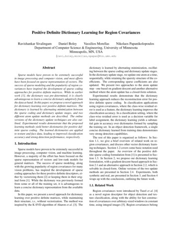
MosaicRelative objective function5.51234510111254.54RandomDictionary onary (%)0.000.818.1311.384.880.232.990.00Table 1: Texture classification results: Error rates (%) on the Brodatz texture dataset - 1-5 are the five 5-texture mosaics, and 10-12are the three 2-texture mosaics.3.5305-NNClassification onsFigure 1: Normalized objective function for the two dictionarylearning algorithms. The dotted lines denote gradient descent andthe continuous lines represent the parallel-sum update. The plotsare shown for K 8 (blue, ), K 15 (red, ) and K 30(green,o).both the training algorithms. The objective function is normalized with respect to that of the original dictionary, sothat the true dictionary will have a total residual error of 1.The parallel-sum update algorithm gives a much better reduction in residual error, compared to the gradient descentupdate. In fact, for K 8 and K 30, there is very littlereduction in the objective function, in the scale of that of theoriginal dictionary. This is due to the fact that the gradientdescent only perturbs the atoms very slightly during the update step, while the parallel-sum update enables the atomsto make huge jumps in the positive definite space.For this experiment as well as the following, the regularization parameter λ is set to 10 3 . For the remainingexperiments, we only use the parallel-sum update for thedictionary learning.3.2. Texture ClassificationIn this section we demonstrate the effect of dictionarylearning in a classification setting for region covariances.We compare the classification performance with learneddictionaries versus dictionaries formed by randomly sampling the training set.We use a subset of the texture mosaics from the popular Brodatz texture dataset [26]. Intensity and gradient features {I, Ix , Iy , Ixx , Iyy } were extracted, and 5 5covariance descriptors were computed over 32 32 blocks(in steps of 16 pixels) in the training images. A separatedictionary was learned for each class, with N 225 training covariances, and K 5 dictionary atoms, per class.Each class dictionary is trained independently, without using training samples from the other class in a discriminativefashion. For the random dictionary, K training points weresampled to fill in the dictionary.The dictionary-based classification is performed as follows - each test point is independently sparse coded witheach class dictionary, using the sparse coding formulationin (2). The residual error due to each class dictionary Ak (x Ak , S), where x is the optimalis denoted as Dldcoefficient vector for that (S, Ak ) pair. The test point is assigned the label k of the class whose dictionary results inthe minimum residual reconstruction error. k arg min Dld(x Ak , S).kTest points were generated by sampling 32 32 blocksfrom the mosaic image in regions of uniform texture. Nospatial regularization of any sort is used in the classificationprocedure, and each test point is labeled independently.The error rates of classification on the five 5-texture mosaics and the three 2-texture mosaics from [26] are shownin Table (1). A k-NN classifier with k 5, retaining theentire training set and using the Riemannian geodesic distance [16], is also shown for comparison. The error rates forthe random dictionary are averaged over 5 runs, each sampling a different dictionary. Note that the purpose of thisexperiment is not to show that covariance dictionaries arethe best classifiers for texture. Rather, the message to takeaway from this experiment is that learning the dictionaryfrom the data provides a substantial performance gain compared to randomly sampled dictionaries, for classificationapplications. This is well-known and accepted for vectordictionary learning, and is demonstrated here for positivedefinite dictionaries.The residual reconstruction error for training the 5-classdictionaries for the first five Brodatz texture mosaics areshown in Figure 2. The objective function is normalizedwith respect to the residual error before training, and henceat iteration 0, the objective function value will be 1. Theplot is to demonstrate that the residual error decrease dueto the parallel-sum update algorithm is also very strong forpractical datasets, and as can be seen, the total residual erroris reduced to almost half of the original.

Relative objective function1Mosaic 1Mosaic 2Mosaic 3Mosaic 4Mosaic 50.90.80.70.60.50246810IterationsFigure 2: Normalized objective function over the parallel-sum dictionary learning iterations for the five 5-texture mosaics. The objective function is the total of residual errors of all 5 dictionaries,at each stage. The plot also shows the objective function valuesduring the dictionary update, after updating each atom.3.3. Face DetectionIn the previous sections we have seen empirically thatthe residual reconstruction error in sparse coding is reducedby learning positive definite dictionaries, and classificationperformance with learned covariance dictionaries is muchbetter than random non-adaptive dictionaries. In this section, we explore the use of the covariance dictionary forface detection. For training, we use images from the FERETface database [27]. 7 images, each from 109 subjects werechosen, and 19 19 covariance descriptors were extracted.The features used were {x, y, I} and Gabor filter responses,g00 (x, y), . . . , g71 (x, y), with 8 orientations and 2 scales.The preprocessing and feature extraction are performed following the approach of Pang et al. [13]. The N 763training covariances were used to train a dictionary of sizeK 38.For testing, images from the GRAZ01 persondataset [28] were processed to extract the same spatial, intensity and Gabor features. Covariance descriptorswere computed over regularly spaced, overlapping windows (60 60, in steps of 15 pixels). All the covarianceswere sparse coded with the learned face dictionary, and theresidual error Dld (Ŝ, S) is used to obtain a detection scoreat each window. The score was computed asscore e 12 Dld (Ŝ,S)σ2d 2,(19)where σd is the bandwidth, computed as the standard deviation of the residual errors in the entire image.The original images and the corresponding face scoreimages are shown in Figure 3. Note that this is a very simple and straightforward application of the region covarianceFigure 3: Face detection results: Sample images (from theGRAZ01 [28] dataset) and their corresponding face score mapsare shown. High values of the face score (white) indicate the likelihood of a face being present, centered at that location. The scoreimages are normalized with respect to their maximum value, forviewing reasons.dictionary learning, with no complex post-processing. Theresidual error from sparse coding an image region with theface dictionary gives us an good estimate of the probability of that window being a face. A mode-finding procedureover this probability map will give the best face detections.Future work includes searching over windows at multiplescales, as well as learning multiscale dictionaries in termsof the covariance descriptors.4. Conclusions & Future WorkIn this paper, we proposed a novel dictionary learningmethodology for positive definite matrices. The dictionarylearning was formulated with an alternating minimizationapproach, and two different atom update procedures wereelaborated. Update equations for online dictionary learning were also presented. Synthetic experiments were shownto validate the learning approaches. Practical computer vision examples were also demonstrated in the classificationas well as detection setting, both indicating the performanceof trained covariance dictionaries.Future work includes analysis of regret bounds for theonline dictionary learning updates, as well as faster methods for coefficient updates. Multiscale extensions either inthe covariance descriptors themselves or in the dictionarylearning procedure would be very suitable for detection applications such as that shown here. While we manually fixthe number of dictionary atoms here, automatic selection ofdictionary size is another interesting issue to be addressed.Scalability of the learning methods to much larger matrixdimensions is also being investigated.

Acknowledgments. This material is based upon worksupported in part by the U.S. Army Research Laboratory and the U.S. Army Research Office under contract#911NF-08-1-0463 (Proposal 55111-CI), and the NationalScience Foundation through grants #IIP-0443945, #CNS0821474, #IIP-0934327, #CNS-1039741, #IIS-1017344,#IIP-1032018, #SMA-1028076, and #IIS-0916750.References[1] R. Sivalingam, D. Boley, V. Morellas, and N. Papanikolopoulos, “Tensor sparse coding for region covariances,” in ECCV2010, Springer Berlin / Heidelberg.[2] K. Guo, P. Ishwar, and J. Konrad, “Action recognition using sparse representation on covariance manifolds of opticalflow,” in 7th IEEE Intl. Conf. on Advanced Video & Signalbased Surveillance, 2010, pp. 188 –195, Aug.-Sept. 2010.[3] M. Aharon, M. Elad, and A. Bruckstein, “K-SVD: An algorithm for designing overcomplete dictionaries for sparse representation,” IEEE Trans. Signal Process., vol. 54, pp. 4311–4322, Nov. 2006.[4] O. Tuzel, F. Porikli, and P. Meer, “Region covariance: A fastdescriptor for detection and classification,” in ECCV 2006,Springer Berlin / Heidelberg.[5] F. Porikli and O. Tuzel, “Fast construction of covariance matrices for arbitrary size image windows,” in IEEE Intl. Conf.on Image Processing, 2006, pp. 1581 –1584, Oct. 2006.[6] H. Wildenauer, B. Micuk, and M. Vincze, “Efficient texturerepresentation using multi-scale regions,” in ACCV 2007,vol. 4843, Springer Berlin / Heidelberg, 2007.[7] O. Tuzel, F. Porikli, and P. Meer, “Pedestrian detection viaclassification on riemannian manifolds,” IEEE Trans. PatternAnal. Mach. Intell., vol. 30, pp. 1713 –1727, Oct. 2008.[8] F. Porikli and T. Kocak, “Robust license plate detection using covariance descriptor in a neural network framework,”in IEEE Intl. Conf. on Video and Signal Based Surveillance,2006, pp. 107–107, Nov. 2006.[9] F. Porikli, O. Tuzel, and P. Meer, “Covariance tracking usingmodel update based on lie algebra,” in IEEE Computer Society Conf. on Computer Vision & Pattern Recognition, 2006,vol. 1, pp. 728 – 735, June 2006.[10] C. Prakash, B. Paluri, S. Nalin Pradeep, and H. Shah, “Fragments based parametric tracking,” in ACCV 2007, SpringerBerlin / Heidelberg.[11] Y. Ma, B. Miller, and I. Cohen, “Video sequence queryingusing clustering of objects appearance models,” in Advancesin Visual Computing, Springer Berlin / Heidelberg.[12] R. Sivalingam, V. Morellas, D. Boley, and N. Papanikolopoulos, “Metric learning for semi-supervised clustering of region covariance descriptors,” in 3rd ACM/IEEE Intl. Conf.on Distributed Smart Cameras, 2009, pp. 1 –8, Aug.-Sept.2009.[13] Y. Pang, Y. Yuan, and X. Li, “Gabor-based region covariancematrices for face recognition,” IEEE Trans. Circuits Syst.Video Technol., vol. 18, pp. 989 –993, July 2008.[14] H. Huo and J. Feng, “Face recognition via AAM and multifeatures fusion on riemannian manifolds,” in ACCV 2009,Springer Berlin / Heidelberg.[15] K. Guo, P. Ishwar, and J. Konrad, “Action change detectionin video by covariance matching of silhouette tunnels,” inIEEE Intl. Conf. on Acoustics Speech & Signal Processing,2010, pp. 1110 –1113, Mar. 2010.[16] X. Pennec, P. Fillard, and N. Ayache, “A riemannian framework for tensor computing,” Int. J. Comput. Vision, vol. 66,pp. 41–66, January 2006.[17] J. Mairal, F. Bach, J. Ponce, G. Sapiro, and A. Zisserman,“Discriminative learned dictionaries for local image analysis,” in IEEE Conf. on Computer Vision & Pattern Recognition, 2008., pp. 1 –8, June 2008.[18] I. Ramirez, P. Sprechmann, and G. Sapiro, “Classificationand clustering via dictionary learning with structured incoherence and shared features,” in IEEE Intl. Conf. on Computer Vision & Pattern Recognition, 2010., pp. 3501 –3508,June 2010.[19] J. Mairal, F. Bach, J. Ponce, and G. Sapiro, “Online dictionary learning for sparse coding,” in 26th Annual Intl. Conf.on Machine Learning, 2009.[20] R. Rubinstein, M. Zibulevsky, and M. Elad, “Double sparsity: Learning sparse dictionaries for sparse signal approxima

Positive Deﬁnite Dictionary Learning for Region Covariances Ravishankar Sivalingam Daniel Boley Vassilios Morellas Nikolaos Papanikolopoulos Department of Computer Science & Engineering, University of Minnesota Minneapolis, MN, USA fravi,boley,morellas,npap