WIXLIB

Using Real Data in an SIR ModelD. SulskyJune 21, 2012In most epidemics it is difficult to determine how many new infectives there areeach day since only those that are removed, for medical aid or other reasons, can becounted. Public health records generally give the number of removed per day, perweek, or per month. So to apply the model to an actual disease, we need to know thenumber removed per unit time, namely, dR/dt as a function of time. Using previousresults, we can obtain an equation for R alone dRR aI a(N0 R S) a N0 R S0 exp , R(0) 0, (1)dtρwhich can only be solved in a parametric way. However this form is not convenient.Of course we can always compute the solution numerically if we know a, b, S0 andN0 . But, usually we don’t know all the parameters. Thus, we try to carry out a bestfit procedure, assuming, of course, that the model actually is a reasonable descriptionof the epidemic.Kermack and McKendrick argued that if the epidemic is not large, R/ρ is small.Using this observation, we can approximate equation (1) as R 1 R 2 dR a N0 R S0 1 ( )dtρ2 ρ (2) S0S0 R 2 a N0 S0 1 R .ρ2ρ2Factoring the right-hand side quadratic in R, we can integrate the equation to get iρ2 h S0αat 1 α tanh φR(t) S0ρ2(3) 2h Stanh 1 ( Sρ0 1)2S0 (N S0 ) i1/20α 1 , φ .ρρ2α1

The removal rate is then given by αat dRaα2 ρ2 sech2 φ ,dt2S02(4)which involves only three parameters, namely aα2 ρ2 /(2S0 ), αb and φ. With epidemicsthat are not large, it is this function of time which we should fit to the Public Healthrecords. On the other hand, if the disease is such that we know the actual number ofthe removed class, then it is R(t) that we should use. If R/ρ is not small, however,we must use the original differential equation for dR/dt.ExamplesBombay Plague Epidemic, 1905-6This epidemic lasted for almost a year. Most of the victims who got the disease died,the number removed per week, that is dR/dt, is approximately equal to the deathsper week. On the basis that the epidemic was not severe (relative to the populationsize), Kermack and McKendrick compared the actual data with (4) and determinedthe best fit for the three parameters and gotdR 890sech2 (0.2t 3.4).dt(5)Figure 1 is from [4] showing the comparison between data and their model. Kermackand McKendrick [4] noteplague in man is a reflection of plague in rats, and that with respect tothe rat (1) the uninfected population was uniformly susceptible; (2) thatall susceptible rats in the island had an equal chance of being infected;(3) that the infectivity, recovery, and death rates were of constant valuethroughout the course of sickness of each rat; (4) that all cases endedfatally or became immune; and (5) that the flea population was so largethat the condition approximated to one of contact infection. None ofthese assumptions are strictly fulfilled and consequently the numericalequation can only be a very rough approximation. A close fit is not tobe expected, and deductions as to the actual values of the various constants should not be drawn. It may be said, however, that the calculatedcurve, which implies that the rates did not vary during the period of theepidemic, conforms roughly to the observed figures.2

Figure 1: Bombay plague data and fit from [4]3

We can also see the threshold effect in this model by examining the removedpopulation (3). At the end of the epidemic (t ), the removed population is iρ2 h S0R( ) 1 α ,S0ρα 22S0 (N0 S0 ) i1/2 1 .ρρ2h S0Since N0 S0 is the initial number of infected individuals, it is reasonable to assumethis number is small compared with S0 and we obtain i2ρ hR( ) S0 ρ .S0If I0 is small then S0 N0 . If N0 is equal to (or less than) ρ, no epidemic can takeplace. If however, N0 slightly exceeds the value ρ then a small epidemic occurs. Ifwe write N0 ρ then R( ) 2 . To a first approximation, the size of theepidemic will be twice the excess if is small compared with N0 . So at the end ofthe epidemic, the population will be just as far below the threshold density, as itinitially was above it.Influenza Epidemic in an English Boarding School, 1978In 1978, anonymous authors sent a note to the British Medical Journal reporting aninfluenza outbreak in a boarding school in the north of England. Figure 2 shows thedata accompanying the note. Table 1 gives values, estimated from the figure, of thenumber of individuals confined to bed each day.The outbreak was in a boys school with a total of 763 boys. Of these, 512 wereconfined to bed during the epidemic which lasted from the 22nd of January to the4th of February. It also seems that one infected boy started the epidemic. Many ofour model assumptions apply to this scenario; however, the epidemic is severe so wecannot use the approximation we made in the last example. Parameter fitting hasto be done by solving the full ordinary differential equations of the SIR model.We can take a simpler approach to get an estimate of the parameters describingthis disease. The epidemic started with one sick boy, with two more getting sick oneday later. Thus, we have I0 1, S0 762 anddS 2 per individual per day.dt dS/dt2a 0.0026.SI762 14

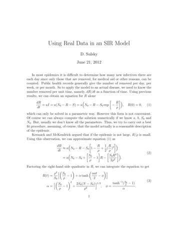
Figure 2: Influenza epidemic in an English Boarding School.Now, b is the rate at which infected people are removed from the population. Thereport says that boys were taken to the infirmary within 1 or 2 days of becomingsick. So crudely, about 1/2 of the infected population was removed each day, orb 0.5 per day. This gives a value of ρ b/a 192. Figure 3 shows a plot of thephase plane with direction field and plots of S(t) and I(t) for these parameters. Wepredict Imax 306 and S( ) 16 from the model.Murray [3] reports performing a careful fit of model parameters using the fullODE model to obtain ρ 202, a 2.18 10 3 /day. The initial conditions are thesame, N0 763, S0 762 and I0 1. We note that these parameter values are closeto our crude estimate and predict a similar course for the disease. The conditions foran epidemic are clearly met according to the model since S0 ρ. The epidemic isalso severe since R/ρ is not always small; R( ) 747 using our ‘crude’ parameters(see Fig. 4).5

800700Boarding School: a 0.0026, b 0.5, S 762, I 002001001005000200400S600800(a)00510time (days)(b)Figure 3: Model predictions compared to data for the English boys school using theSIR model with a 0.0026, b 0.5, S0 762 and I0 1.615

Day 312145Table 1: Boarding School Data for Individuals Confined to BedBoarding School: a 0.0026, b 0.5, S 762, I 02468time (days)101214Figure 4: Model predictions compared to data for the English boys school using theSIR model with a 0.0026, b 0.5, S0 762 and I0 1.7

Plague Outbreak in Eyam Village, 1665-66In a wonderfully altruistic incident, the village of Eyam, England sealed itself off in1665-66 when the plague was discovered, so as to prevent it spreading to neighboringvillages. There is a museum in Eyam that tells the story ( http://www.eyammuseum.demon.co.uk/). The villagers were successful in controlling the spread to other villages, but by theend of the epidemic only 83 of the original population of 350 survived. So we knowS0 350 and S( ) 83, but how do we obtain other information about parametersfor a model? The discussion in this section is based heavily on [6].The source of the plague in Eyam is attributed to the Great Plague of London(1664-1666) in which one sixth of the population succumbed to the disease. A tailorin Eyam received cloth from London which was infected with plague-carrying ratfleas that can produce plague in humans by biting their victims. The first victimwas his assistant, George Viccars, who was buried September 7, 1665. Thereafter, theplague started to infect other victims as shown in Table 2. At this point the plague1665 September 6 deathsOctober23 deathsNovember7 deathsDecember9 deaths1666 January5 deathsFebruary8 deathsMarch6 deathsApril9 deathsMay4 deathsTable 2appeared to be diminishing. But at the start of summer, the plague re-establisheditself. The next 5 months of deaths are shown in Table 3. Even though the datesand numbers are reported as deaths, they were actually burial dates. It is believedthat burials were almost immediate for health reasons. However, toward the end ofthe outbreak there were no family members to bury the dead and burials might havebeen delayed. Marshall Howe was known to be a self-appointed grave digger whopaid himself from the belongings of the dead.The original strain of the Eyam plague is believed to be bubonic - from the ratfleas. It is believed that the outbreak did not continue in this form but turned atleast partially to pneumonic, i.e. infected directly from person to person. This belief8

1666 hsdeathsdeathsdeathsTable 3is based on the fact that even though infected rodent fleas are temporarily importantin the causation of bubonic plague in man, the continued existence of this form ofthe disease depends on the persistence of infected rodents. In this case, the originalrodent was 150 miles away.The SIR model is reasonable for this plague epidemic for the following reasons1. The transmission of the plague is a rapidly spreading infectious disease.2. The complete isolation of the village keeps N fixed. (This assumption is reallyonly approximate since some wealthy villagers and some children fled. A fewbirths and natural deaths were also recorded. However, the total populationfor the purposes of the model can be estimated at the outbreak time as thesum of final survivors and those who died during the plague. These figures areknown.)3. Only three cases of infected individuals are known to have survived. (One ofthese was Marshall Howe who presumable built up some immunity by beinginvolved with repeated burials.) For the purpose of the model we can assume infected people were removed from the population by death. The time-dependentremoved population is measurable from the list of dead.The SIR model predicts a single peak Imax given byImax N0 ρ ρ lnρ.S0(6)However, the Eyam data contain at least two local infection peaks. We noticedthe milder outbreak initially followed by more devastating later effects. Raggett [6]argues we can apply the SIR model starting in May or June, 1666. Then there isone peak in the data and the majority of the deaths are included. In the reference,Raggett starts on June 18. He also uses a time measurement of 15 1/2 days. The listof dead provides data for the deceased and removed (cumulative deceased). Table 49