WIXLIB

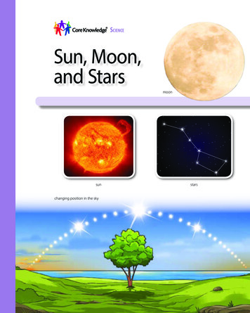
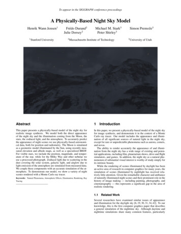
To appear in the SIGGRAPH conference proceedingsstar thlightairglowMilky phere A irglow layerhorMoonlocalzenithFigure 4: Coordinate systems. Left: equatorial (α, δ) and ecliptic(λ, β). Right: Local coordinates (A, h) for an observer at longitudelon and latitude lat.Figure 3: Components of the night sky model.latitude is the altitude angle h above the horizon, and the longitude, or azimuth A, is measured eastward from the south direction(Figure 4).The two other systems are centered on the Earth but do not depend on its rotation. They differ by their vertical axis, either theNorth pole (and thus the axis of rotation of the Earth) for the equatorial system, or the normal to the ecliptic, the plane of the orbit ofthe Earth about the Sun, for the ecliptic system (Figures 1 and 4).The Earth’s rotational axis remains roughly parallel as the Earthorbits around the Sun (the angle between the ecliptic and the Equator is about 23.44 ). This means that the relationship between theangles of the two systems does not vary. In both cases, the reference for the longitude is the Vernal Equinox, denoted , whichcorresponds to the intersection of the great circles of the Equatorand the ecliptic (Figure 4).However, the direction of the axis of the Earth is not quite constant. Long-term variations known as precession and short-term oscillations known as nutations have to be included for high accuracy,as described in the Appendix. Stars. The appearance of the brightest stars is simulated usingdata that takes into account their individual position, magnitude and temperature. Planets are displayed similarly, albeitby first computing their positions. Star clouds — elementsthat are too dim to observe as individual stars but collectivelyproduce visible light — including the Milky Way, are simulated using a high resolution photograph of the night sky processed to remove the bright stars. Illumination from stars istreated differently, using a simple constant model. Other astronomical elements. Zodiacal light, atmosphericairglow, diffuse galactic light, and cosmic lights are simulatedusing measured data. Atmospheric scattering. We simulate multiple scattering inthe atmosphere due to both molecules and aerosols.3Astronomical Positions3.2We introduce classical astronomical formulas to compute the position of various celestial elements. For this, we need to reviewastronomical coordinate systems. This section makes simplifications to make this material more accessible. For a more detaileddescription, we refer the reader to classic textbooks [7, 10, 23, 24]or to the year’s Astronomical Almanac [44].All of the formulas in the Appendix have been adapted from highaccuracy astronomical formulas [23]. They have been simplified tofacilitate subsequent implementation, as computer graphics applications usually do not require the same accuracy as astronomicalapplications. We have also made conversions to units that are morefamiliar to the computer graphics community. Our implementationusually uses higher precision formulas, but the error introduced bythe simplifications is lower than 8 minutes of arc over five centuries.3.1Position of the SunThe positions of the Sun and Moon are computed in ecliptic coordinates (λ, β) and must be converted using the formulas in Appendix.We give a brief overview of the calculations involved. Formulas exhibit a mean value with corrective trigonometric terms (similar toFourier series).The ecliptic latitude of the Sun should by definition be βSun 0. However, small corrective terms may be added for very highprecision, but we omit them since they are below 1000 .3.3The MoonThe formula for the Moon is much more involved because of theperturbations caused by the Sun. It thus requires many correctiveterms. An error of 1 in the Moon position corresponds to as muchas 2 diameters. We also need to compute the distance dMoon , whichis on average 384 000 km. The orbital plane of the Moon is inclinedby about 5 with respect to the ecliptic. This is why solar and lunareclipses do not occur for each revolution and are therefore rare.The Moon orbits around the Earth with the same rotational speedas it rotates about itself. This is why we always see nearly thesame side. However, the orbit of the Moon is not a perfect circlebut an ellipse (eccentricity about 1/18), and its axis of revolutionis slightly tilted with respect to the plane of its orbit (Figure 5).For this reason, about 59% of the lunar surface can be seen fromthe Earth. These apparent oscillations are called librations and areCoordinate SystemsThe basic idea of positional astronomy is to project everything ontocelestial spheres. Celestial coordinates are then spherical coordinates analogous to the terrestrial coordinates of longitude and latitude. We will use three coordinate systems (Figure 4) — two centered on the Earth (equatorial and ecliptic) and one centered on theobserver (horizon). Conversion formulas are given in the Appendix.The final coordinate system is the local spherical frame of theobserver (horizon system). The vertical axis is the local zenith, the3

To appear in the SIGGRAPH conference proceedingstrue axis orthogonalof rotation axisexact circletrue orbitEarthnormalqiqr igure 6: Angle for the BRDF of the Moon.Figure 5: (a) Librations of the Moon are due to the eccentricity ofits orbit and to the tilt of its axis of rotation. (b) Angle for the BRDFof the Moon.Accuracy is not crucial for earthshine except for the new Moon,so we simply use the percentage of lit Earth visible from the Moonand multiply it by the intensity of the full earthshine, which isW0.19 m2 . Given the Earth phase, that is, the angle π ϕ betweenthe Moon and the Sun as seen from the Earth (the opposite of theMoon phase ϕ), we obtain [46]:included in our model as a result of our direct modeling approach.(See the Appendix for formulas.)3.4hπ ϕπ ϕπ ϕ iEem 0.19 0.5 1 sin() tan() ln(cot())224(1)Position of StarsFor the stars, we used the Yale Bright Star Catalog [14]. It containsabout 9000 stars, including the roughly 6000 visible to the nakedeye. The stellar positions are given in equatorial coordinates. Thecatalogue contains the position for 2000 A.D. and the proper motion of stars, caused by their rectilinear motion through space. Theposition of a star for a given date is then computed using a linear approximation, usually in rectangular coordinates (the apparent motion can be neglected if the date is less than 5 centuries from 2000A.D.). The positions of the planets are computed using formulassimilar to those used for the Moon and the Sun [23].44.2The Moon has a low albedo and a reddish color, and it exhibitsbackscattering reflection (it is much brighter at full Moon) [11].Furthermore, the apparent disc of the full Moon has a remarkablephotometric property: its average brightness at the center is thesame as at the edge [11]. The Moon is therefore said to exhibitno limb darkening. This can be explained by the pulverized nature of its surface. We use the complete Hapke-Lommel-Seeligermodel of the reflectance function of the Moon, which provides agood approximation to the real appearance and a good fit to measured data [12]. The BRDF f consists of a retrodirective functionB and a scattering function S. As the BRDF of the Moon is ratheruniform, but the albedo is variable, we model them independently.We multiply the BRDF by the albedo and by the spectrum of theMoon.The geometry for the BRDF is summarized in Figure 6. ϕ isthe lunar phase angle (angle Sun-Earth as seen from the Moon, orequivalently for our purpose, the angle between incident and reflected light). θr is the angle between the reflected light and thesurface normal; θi is the angle between the incident light and thesurface normal.Note that to compute the contribution of the earthshine, the Sunhas to be replaced by the Earth using Equation 1 for the intensity.ϕ is then null by definition.The BRDF, f , of the Moon can be computed with:MoonlightThe large-scale topography of the Moon is visible from the Earth’ssurface, so we render its direct appearance using a geometric modelcontaining elevation and albedo illuminated by two directional lightsources, the Earth and the Sun.4.1BRDF of the MoonModeling the MoonTo model the Moon accurately, we use the positions computed inthe previous section and measured data of the lunar topography andalbedo [27]. The Moon is considered a poor reflector: on averageonly 7.2% of the light is reflected [20]. The albedo is used to modulate a BRDF model, which we present in the next section. Theelevation is measured with a precision of a quarter of a degree inlongitude and latitude (1440 720), and the albedo map has size800 400.The Moon is illuminated by the Sun, which can be treated as adirectional light source. We use the positions of the Moon and Sunto determine the direction of illumination. The Sun is modeled as ablack body at temperature 5900K (see Appendix for conversion),Wand power 1905 m2 . The Sun appears about 1.44 times brighterfrom the Moon than from the surface of the Earth because of theabsence of atmosphere. We do not include the Earth as an occluder,which means we cannot simulate lunar eclipses. This could easilybe done by modeling the Sun as a spherical light source to simulatepenumbra.The faint light visible on the dark side of the Moon when it is athin crescent is known as earthshine. Earthshine depends stronglyon the phase of the Earth. When the Earth is full (at new Moon), itcasts the greatest amount of light on the Moon, and the earthshineis relatively bright and easily observed by the naked eye. We modelearthshine explicitly by including the Earth as a second light sourcefor the Moon surface.f (θi , θr , ϕ) 12B(ϕ, g)S(ϕ).3π1 cos θr / cos θiThe retrodirective function B(ϕ, g) is given by ϕ2 tan1 e g/ tan ϕ3 e g/ tan ϕ ,2gB(ϕ, g) 1,(2)ϕ π/2ϕ π/2,(3)where g is a surface density parameter which determines the sharpness of the peak at the full Moon. We use g 0.6, although valuesbetween 0.4 (for rays) and 0.8 (for craters) could be used.The scattering law S for individual objects is given by [12]: 2sin ϕ (π ϕ ) cos ϕ 1 t 1 cos ϕ , (4)S(ϕ) π2where t introduces a small amount of forward scattering that arisesfrom large particles that cause diffraction [37]. t 0.1 is a good fitto Rougier’s measurements [16] of the light from the Moon.4

To appear in the SIGGRAPH conference proceedingsThe spectrum of the Moon is distinctly redder than the Sun’sspectrum. Indeed, the lunar surface consists of a layer of a porouspulverized material composed of particles larger than the wavelengths of visible light. As a consequence and in accordance withthe Mie theory [45], the albedo is approximately twice as large forred (longer wavelengths) light than for blue (shorter wavelengths)light. In practice, we use a spectral reference that is a normalizedlinear ramp (from 70% at 340nm to 135% at 740nm). In addition,light scattered from the lunar surface is polarized, but we do notinclude polarization in our model. Figure 7 demonstrates our Moonmodel for various conditions.4.3stars with a stellar magnitude up to approximately 6. However, thisis the visible magnitude, which takes into account the atmosphericscattering. Since we simulate atmospheric scattering, we must discount this absorption, which accounts for 0.4 magnitude:Es0 100.4( mv 19 0.4)For illumination coming from the Moon, it is sufficient to use a simple directional model since the Moon is very distant. This moreoverintroduces less variance in the illumination integration.Using the Lommel-Seeliger law [46], the irradiance Em fromthe Moon at phase angle ϕ and a distance d can be expressed as:22 C rm3 d2 Eem Esm 1 sinϕ2tanϕ2log cotϕ 4,(5)where rm is the radius of the Moon, Esm is the irradiance from theSun at the surface of the Moon, and Eem is the earthshine contribution as computed from Equation 1. Recall that the phase angle ofthe Moon with respect to earthshine is always null. The normalizing constant C is the average albedo of the Moon (C 0.072).5To compute spectral irradiance from a star given Tef f , we firstcompute a non-spectral irradiance value from the stellar magnitudeusing Equation 7. We then use the computed value to scale a normalized spectrum based on Planck’s radiation law for black bodyradiators [39]. The result is spectral irradiance.In the color pages (Figure 9) we have rendered a close-up ofstars. We use the physically-based glare filter by Spencer et al. [41]as a flare model for the stars. This model fits nicely with the observations by Navarro and Losada [28] regarding the shape of stars asseen by the human eye.Figure 10 is a time-lapse rendering of stars. Here we have simulated a camera and omitted the loss of color by a human observer.The colors of the stars can be seen clearly in the trails. Notice, alsothe circular motion of the stars due to the rotation of the Earth.StarlightStars are important visual features in the sky. We use actual starpositions (as described in Section 3.4), and brightnesses and colors from the same star catalogue [14]. In this section, we describehow stars are included in our model, present the calculation of theirbrightness and chromaticity, and finally, discuss the illuminationcoming from stars.5.35.1Rendering StarsIllumination from StarsEven though many stars are not visible to the naked eye, there is acollective contribution from all stars when added together. We useWa constant irradiance of 3 · 10 8 m2 [38] to account for integratedstarlight.Stars are very small, and it is therefore not practical to use explicitray tracing to render them as rays would easily miss them. Instead,we use an image-based approach in which a separate star image isgenerated and composited using an alpha image that models attenuation in the atmosphere. The use of the alpha image ensures that theintensity of the stars is correctly reduced due to scattering and absorption in the atmosphere. The alpha map records for every pixelthe visibility of objects beyond the atmosphere. It is generated bythe ray tracer as a secondary image. Each time a ray from the camera leaves the atmosphere, the transmitivity is stored in the alphaimage. The star image is multiplied by the alpha image and addedto the rendered image to produce the final image.For star clusters, such as the Milky Way, where individual starsare not visible, we use a high resolution (14400x7200) photographic mosaic of the Night Sky [25]. The brightest stars wereremoved using pattern-matching and median filtering.5.2(7)The color of the star is not directly available as a measured spectrum. Instead, astronomers have established a standard series ofmeasurements in particular wave-bands. A widely used UBV system introduced by Johnson [18] isolates bands of the spectrum inthe blue intensity B, yellow-green intensity V , and ultra-violet intensity U . The difference B V is called the color index of a star,which is a numerical measurement of the color. A negative value ofB V indicates a more bluish color, while a positive value indicatesa redder hue. U BV is not directly useful for rendering purposes.However, we can use the color index to estimate a star’s temperature [33, 40]:7000KTef f .(8)B V 0.56Illumination from the MoonEm (ϕ, d) W.m26Other ElementsA variety of phenomena affect the appearance of the night sky insubtle ways. While one might assume the sky itself is colored onlyby scattered light in the atmosphere, that is in fact only one of fourspecific sources of diffuse visible color in the night sky. The otherthree are zodiacal light, airglow, and galactic/cosmic light. We include all of these in our model. These effects are especially important on moonless nights, when a small change in illumination candetermine whether an object in the scene is visible or invisible.6.1Color and Brightness of StarsA stellar magnitude describes the apparent star brightness. Giventhe visual magnitude, the irradiance at the Earth is [21]:Zodiacal LightThe Earth co-orbits with a cloud of dust around the Sun. Sunlightscatters from this dust and can be seen from the Earth as zodiacallight [5, 36]. This light first manifests itself in early evening as adiffuse wedge of light in the southwestern horizon and graduallybroadens with time. During the course of the night the zodiacallight becomes wider and more upright, although its position relativeto the stars shifts only slightly [2].W.(6)m2For the Sun, mv 26.7; for the full Moon, mv 12.2; andfor Sirius, the brightest star, mv 1.6. The naked eye can seeEs 100.4( mv 19)5

To appear in the SIGGRAPH conference proceedings7The structure of the interplanetary dust is not well-understood.To to simulate zodiacal light we use a table with measured values [38]. Whenever a ray exits the atmosphere, we convert the direction of the ray to ecliptic polar coordinates and perform a bilinearlookup in the table. This works well since zodiacal light changesslowly with direction and has very little seasonal variation. A resultof our zodiacal light model is illustrated Figure 8.6.2We implemented our night sky model in a Monte Carlo ray tracerwith support for spectral sampling. We used an accurate spectralsampling with 40 evenly-spaced samples from 340nm to 740nm toallow for precise conversion to XYZV color space for tone mapping, as well as for accurately handling the wavelength dependentRayleigh scattering of the sky. Simpler models could be used aswell, at the expense of accuracy.Because our scenes are at scotopic viewing levels (rod vision),special care must be taken with tone mapping. We found thehistogram-adjustment method proposed by Ward et al. [22] to workbest for the very high dynamic range night images. This method“discounts” the empty portions of the histogram of luminance, andsimulates both cone (daylight) and rod (night) vision as well as lossof acuity. Another very important component of our tone-mappingmodel is the blue-shift (the subjective impression that night scenesexhibit a bluish tint). This phenomena is supported by psychophysical data [15] and a number of techniques can be used to simulateit [8, 17, 43]. We use the technique for XYZV images as describedin [17].Many features of our model have been demonstrated through thepaper. Not all of the elements can be seen simultaneously in oneimage. In particular, the dimmest phenomena such as zodiacal lightare visible only for moonless nights. Phenomena such as airglowand intergalactic light are present only as faint background illumination. Nonetheless, all these components are important to give arealistic impression of the night sky. The sky is never completelyblack.Our experimental results are shown in the two color pages at theend of the paper. The captions explain the individual images. Allthe images were rendered on a dual PIII-800 PC, and the renderingtime for most of the individual images ranged from 30 seconds to2 minutes. It may seem surprising that multiple scattering in theatmosphere can be computed this quickly. The main reason for thisis that multiple scattering often does not contribute much and assuch can be computed with low accuracy — as also demonstratedin [29]. The only images that were more costly to render are theimages with clouds; we use path tracing of the cloud media and thisis quite expensive. As an example the image of Little Matterhorn[35] with clouds (Figure 13) took 2 hours to render.A very important aspect of our images is the sense of night. Thisis quite difficult to achieve, and it requires carefully ensuring correct physical values and using a perceptually based tone-mappingalgorithm. This is why we have stressed the use of accurate radiometric values in this paper. For a daylight simulation it is lessnoticeable if the sky intensity is wrong by a factor two, but in thenight sky all of the components have to work together to form animpression of night.AirglowAirglow is faint light that is continuously emitted by the entire upper atmosphere with a main concentration at an elevation of approximately 110 km. The upper atmosphere of the Earth is continually being bombarded by high energy particles, mainly fromthe Sun. These particles ionize atoms and molecules or dissociatemolecules and in turn cause them to emit light in particular spectrallines (at discrete wavelengths). As the emissions come primarilyfrom Na and O atoms as well as molecular nitrogen and oxygen theemission lines are easily recognizable. The majority of the airglowemissions occur at 557.7nm (O-I), 630nm (O-I) and a 589.0nm 589.6nm doublet (Na-I). Airglow is the principal source of light inthe night sky on moonless nights.Airglow is integrated into the simulation by adding an activelayer to the atmosphere (altitude 80km) that contributes a spectralWin-scattered radiance (5.1 · 10 8 m2 , 3 peaks, at 557.7nm, 583.0nmand 630.0nm).6.3Diffuse Galactic Light and Cosmic LightDiffuse galactic light and cosmic light are the last components ofthe night sky that we include in our model. These are very faintW(see Figure 2) and modeled as a constant term (1 · 10 8 m2 ) that isadded when a ray exits the atmosphere.6.4Implementation and ResultsAtmosphere ModelingMolecules and aerosols (dust, water drops and other si

of naturally illuminated night scenes and their prominent role in the history of image making — including painting, photography, and cinematography — this represents a significant gap in the area of realistic rendering. 1.1 Related W