WIXLIB

Investors are typically concerned with long-term performance when comparing alternativeinvestments. GM is considered a superior measure of the long-term mean rate of return becauseit indicates the compound annual rate of return based on the ending value of the investmentversus its beginning value. Specifically, using the prior example, if we compounded 3.353percent for three years, (1.03353), we would get an ending wealth value of 1.104.Although the arithmetic average provides a good indication of the expected rate of return for aninvestment during a future individual year, it is biased upward if you are attempting to measurean asset’s long-term performance. This is obvious for a volatile security. Consider, for example,a security that increases in price from 50 to 100 during year 1 and drops back to 50 duringyear 2.The annual HPYs would be:This would give an AM rate of return of:This investment brought no change in wealth and therefore no return, yet the AM rate of return iscomputed to be 25 percent.The GM rate of return would be:This answer of a 0 percent rate of return accurately measures the fact that there was no change inwealth from this investment over the two-year period. When rates of return are the same for allyears, the GM will be equal to the AM. If the rates of return vary over the years, the GM willalways be lower than the AM. The difference between the two mean values will depend on theyear-to-year changes in the rates of return. Larger annual changes in the rates of return—that is,more volatility—will result in a greater difference between the alternative mean values.An awareness of both methods of computing mean rates of return is important because publishedaccounts of investment performance or descriptions of financial research will use both the AMand the GM as measures of average historical returns.10

1.2.3 Calculating Expected Rates of ReturnRisk is the uncertainty that an investment will earn its expected rate of return. In the examplesin the prior section, we examined realized historical rates of return. In contrast, an investor whois evaluating a future investment alternative expects or anticipates a certain rate of return.The investor might say that he or she expects the investment will provide a rate of return of 10percent, but this is actually the investor’s most likely estimate, also referred to as a pointestimate. Pressed further, the investor would probably acknowledge the uncertainty of this pointestimate return and admit the possibility that, under certain conditions, the annual rate of returnon this investment might go as low as 10 percent or as high as 25 percent. The point is, thespecification of a larger range of possible returns from an investment reflects the investor’suncertainty regarding what the actual return will be. Therefore, a larger range of possible returnsimplies that the investment is riskier.An investor determines how certain the expected rate of return on an investment is by analyzingestimates of possible returns. To do this, the investor assigns probability values to all possiblereturns. These probability values range from zero, which means no chance of the return, to one,which indicates complete certainty that the investment will provide the specified rate of return.These probabilities are typically subjective estimates based on the historical performance of theinvestment or similar investments modified by the investor’s expectations for the future.As an example, an investor may know that about 30 percent of the time the rate of return on thisparticular investment was 10 percent. Using this information along with future expectationsregarding the economy, one can derive an estimate of what might happen in the future.The expected rate of return from an investment is: is the sum of the products of each possibleoutcome times its associated probability—it is a weighted average of the various possibleoutcomes, with the weights being their probabilities of occurrence:Expected Return E(R i )n (Probability of Return) (PossibleReturn)i 1 nExpected rate of return r Pi r i .i 1 Where the number of possible outcomes is virtually unlimited, continuous probabilitydistributions are used in determining the expected rate of return of the event.The tighter, or more peaked, the probability distribution, the more likely it is that theactual outcome will be close to the expected value, and, consequently, the less likely it is11

that the actual return will end up far below the expected return. Thus, the tighter theprobability distribution, the lower the risk assigned to a stock.Risk aversion: The assumption that most investors will choose the least risky alternative, allelse being equal and that they will not accept additional risk unless they are compensated in theform of higher return Most investors are risk averse. This means that for two alternatives with the sameexpected rate of return, investors will choose the one with the lower risk. No investment will be undertaken unless the expected rate of return is high enough tocompensate the investor for the perceived risk of the investment.Illustration- Expected rate of return: Let us begin our analysis of the effect of risk with anexample of perfect certainty wherein the investor is absolutely certain of a return of 5 percent.Let us begin our analysis of the effect of risk with an example of perfect certainty wherein theinvestor is absolutely certain of a return of 5 percent. Exhibit 1.1 illustrates this situation.Perfect certainty allows only one possible return, and the probability of receiving that return is1.0. Few investments provide certain returns and would be considered risk-free investments.In the case of perfect certainty, there is only one value for PiRi:E(Ri) (1.0)(0.05) 0.05 5%Probability Distributiona probability distribution gives all the possible outcomes with the chance, or probability, eachoutcome will occurFigure 1.1 Probability distribution for risk free investment1.000.800.600.400.200.00-5%0%5% 10% 15%In an alternative scenario, suppose an investor believed an investment could provide severaldifferent rates of return depending on different possible economic conditions. As an example, ina strong economic environment with high corporate profits and little or no inflation, the investor12

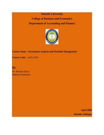
might expect the rate of return on common stocks during the next year to reach as high as 20percent. In contrast, if there is an economic decline with a higher-than-average rate of inflation,the investor might expect the rate of return on common stocks during the next year to be 20percent. Finally, with no major change in the economic environment, the rate of return during thenext year would probably approach the long-run average of 10 percent.The investor might estimate probabilities for each of these economic scenarios based on pastexperience and the current outlook as follows:Economic ConditionsReturnProbabilityRate ofStrong economy, no inflation0.150.20Weak economy, above-average inflation0.15 0.20No major change in economy0.700.10This set of potential outcomes can be visualized as shown in Exhibit 1.2.The computation of the expected rate of return [E(Ri)] is as follows:E(Ri) [(0.15)(0.2) (0.15)(-0.2) (0.7)(0.1)] 0:07Obviously, the investor is less certain about the expected return from this investment than aboutthe return from the prior investment with its single possible return.A third example is an investment with 10 possible outcomes ranging from 40 percent to 50percent with the same probability for each rate of return. A graph of this set of expectationswould appear as shown in Exhibit 1.3.In this case, there are numerous outcomes from a wide range of possibilities. The expected rateof return [E(Ri)] for this investment would be:E(Ri) [(0.10)(-0.4) (0.10)(-0.3) (0.1)(-0.2) (0.10)(-0.1) (0.10)(0.00) (0.1)(0.1) (0.10)(0.20) (0.1)(0.3) (0.1)(0.4) (0.10)(0.50)] [(-0.04) (-0.03) (-0.02) (-0.01) (0.00) (0.01) (0.02) (0.03) (0.04) (0.05) 0.05 5%13

The expected rate of return for this investment is the same as the certain return discussed in thefirst example; but, in this case, the investor is highly uncertain about the actual rate of return.This would be considered a risky investment because of that uncertainty.We would anticipate that an investor faced with the choice between this risky investment and thecertain (risk-free) case would select the certain alternative. This expectation is based on thebelief that most investors are risk averse, which means that if everything else is the same, theywill select the investment that offers greater certainty (i.e., less risk).Figure 1.2: Probability Distribution for Risky Investment with Three Possible Rates re 1.3: Probability Distribution for Risky Investment with 10 Possible Rates of Return1.000.800.600.400.200.00-40% -20%0%20%1.2.4 Measures the Risk of the Expected Rates of Return1440%

We have shown that we can calculate the expected rate of return and evaluate the uncertainty, orrisk, of an investment by identifying the range of possible returns from that investment andassigning each possible return a weight based on the probability that it will occur. Although thegraphs help us visualize the dispersion of possible returns, most investors want to quantify thisdispersion using statistical techniques. These statistical measures allow you to compare thereturn and risk measures for alternative investments directly. Two possible measures of risk(uncertainty) have received support in theoretical work on portfolio theory: the variance and thestandard deviation of the estimated distribution of expected returns.nVariance ( probability (possible rate of return-expected rate of return)2i 1Standard Deviation is the square root of the varianceStd n P [Ri 1ii- E(R i )]2Std 2.The standard deviation is a probability-weighted average deviation from the expected value,and it gives you an idea of how far above or below the expected value the actual value islikely to be.Question: Compute the variance and Standard deviation for the three examples aboveAns: 1.The variance for the perfect-certainty example would be: 02.This gives an expected return [E(Ri)] of 7 percent. The dispersion of this distribution asmeasured by variance is:15

The variance (σ2) is equal to 0.0141. The standard deviation is equal to the square root of thevariance:Consequently, the standard deviation for the preceding example would be:In this example, the standard deviation is approximately 11.87 percent. Therefore, you coulddescribe this distribution as having an expected value of 7 percent and a standard deviation of11.87 percent.Coefficient of VariationThe variance and standard deviation are absolute measures of dispersion. That is, they can beinfluenced by the magnitude of the original numbers. To compare series with greatly differentvalues, you need a relative measure of dispersion. A measure of relative dispersion is thecoefficient of variation, which is defined as: Because lower risk is preferred to higher risk andhigher return is preferred to lower return, an investment with a lower coefficient of variation,CV, is preferred to aninvestment with a higher CVA larger value indicates greater dispersion relative to the arithmetic mean of the series. For theprevious example, the CV would be:16

It is possible to compare this value to a similar figure having a markedly different distribution.As an example, assume you wanted to compare this investment to another investment that had anaverage rate of return of 10 percent and a standard deviation of 9 percent. The standarddeviations alone tell you that the second series has greater dispersion (9 percent versus 7.56percent) and might be considered to have higher risk. In fact, the relative dispersion for thissecond investment is much less.Considering the relative dispersion and the total distribution, most investors would probablyprefer the second investment.1.2.5 Measuring the Risk of Historical Rates of ReturnIn many instances, you might want to compute the variance or standard deviation for a historicalseries in order to evaluate the past performance of the investment. To measure the risk for aseries of historical rates of returns, we use the same measures as for expected returns (varianceand standard deviation) except that we consider the historical holding period yields (HPYs) asnfollows: 2 [ HPYi E ( HPY) 2/ni 1Assume that you are given the following information on annual rates of return (HPY) forcommon stocks listed on the New York Stock Exchange (NYSE):In this case, we are not examining expected rates of return but actual returns. Therefore, weassume equal probabilities, and the expected value (in this case the mean value, R) of the seriesis the sum of the individual observations in the series divided by the number of observations, or0.04 (0.20/5). The variances and standard deviations are:17

We can interpret the performance of NYSE common stocks during this period of time by sayingthat the average rate of return was 4 percent and the standard deviation of annual rates of returnwas 7.56 percent.1.3 DETERMINANTS OF REQUIRED RATES OF RETURNRecall that the selection process of an investment involves finding securities that provide a rateof return that compensates you for: (1) the time value of money during the period of investment,(2) the expected rate of inflation during the period, and (3) the risk involved.The summation of these three components is called the required rate of return. This is theminimum rate of return that you should accept from an investment to compensate you fordeferring consumption. Because of the importance of the required rate of return to the totalinvestment selection process, this section contains a discussion of the three components and whatinfluences each of them.The analysis and estimation of the required rate of return are complicated by the behavior ofmarket rates over time. First, a wide range of rates is available for alternative investments at anytime. Second, the rates of return on specific assets change dramatically over time. Third, thedifference between the rates available (that is, the spread) on different assets changes over time.The real risk-free rate (RRFR) is the basic interest rate, assuming no inflation and nouncertainty about future flows. An investor in an inflation-free economy who knew withcertainty what cash flows he or she would receive at what time would demand the RRFR on aninvestment. Earlier, we called this the pure time value of money, because the only sacrifice theinvestor made was deferring the use of the money for a period of time. This RRFR of interest isthe price charged for the exchange between current goods and future goods.Two factors, one subjective and one objective, influence this exchange price. The subjectivefactor is the time preference of individuals for the consumption of income. When individualsgive up 100 of consumption this year, how much consumption do they want a year from now tocompensate for that sacrifice? The strength of the human desire for current consumptioninfluences the rate of compensation required. Time preferences vary among individuals, and themarket creates a composite rate that includes the preferences of all investors. This composite rate18

changes gradually over time because it is influenced by all the investors in the economy, whosechanges in preferences may offset one another.The objective factor that influences the RRFR is the set of investment opportunities available inthe economy. The investment opportunities are determined in turn by the long-run real growthrate of the economy. A rapidly growing economy produces more and better opportunities toinvest funds and experience positive rates of return. A change in the economy’s long-run realgrowth rate causes a change in all investment opportunities and a change in the required rates ofreturn on all investments. Just as investors supplying capital should demand a higher rate ofreturn when growth is higher; those looking for funds to invest should be willing and able to paya higher rate of return to use the funds for investment because of the higher growth rate. Thus, apositive relationship exists between the real growth rate in the economy and the RRFR.Factors Influencing the Nominal Risk-Free Rate (NRFR)when we discuss rates of interest, we need to differentiate between real rates of interest thatadjust for changes in the general price level, as opposed to nominal rates of interest that arestated in money terms. That is, nominal rates of interest that prevail in the market are determinedby real rates of interest, plus factors that will affect the nominal rate of interest, such as theexpected rate of inflation and the monetary environment.Nominal RFR (1 Real RFR) x (1 Expected Rate of Inflation) - 1Rearranging the formula, you can calculate the RRFR of return on an investment as follows: (1 Nominal RFR) (1 Rate of Inflation) 1 Example: assume that the nominal return on U.S. government T-bills was 9 percent during agiven year, when the rate of inflation was 5 percent. What would be the RRFR of return on thisT-bills ?RRFR [(1 0.09)/(1 0.05)] – 1 1.038 – 1 0.038 3.8%Risk PremiumA risk-free investment was defined as one for which the investor is certain of the amount andtiming of the expected returns. The returns from most investments do not fit this pattern. Aninvestor typically is not completely certain of the income to be received or when it will bereceived. Investments can range in uncertainty from basically risk-free securities, such as T-bills,19

to highly speculative investments, such as the common stock of small companies engaged inhigh-risk enterprises.Most investors require higher rates of return on investments if they perceive that there is anyuncertainty about the expected rate of return. This increase in the required rate of return over theNRFR (Nominal Risk Free Rate) is the risk premium (RP). Although the required risk premiumrepresents a composite of all uncertainty, it is possible to consider several fundamental sourcesof uncertainty.Major Sources of Uncertainty: business risk, financial risk (leverage), liquidity risk, exchange rate risk, and Country (political) risk. The standard deviation of returns is referred to as a measure of the security’s total risk, whichconsiders the individual stock by itself—that is, it is not considered as part of a portfolio.Markowitz and Sharpe indicated that investors should use an external market measure of risk.Under a specified set of assumptions, all rational, profit maximizing investors want to hold acompletely diversified market portfolio of risky assets, and they borrow or lend to arrive at a risklevel that is consistent with their risk preferences. Under these conditions, the relevant riskmeasure for an individual asset is its co movement with the market portfolio. This co movement,which is measured by an asset’s covariance with the market portfolio, is referred to as an asset’ssystematic risk, the portion of an individual asset’s total variance attributable to the variabilityof the total market portfolio. In addition, individual assets have variance that is unrelated to themarket portfolio (that is, it is nonmarket variance) that is due to the asset’s unique features. Thisnonmarket variance is called unsystematic risk,

Text and reference books Text Book: Chandra, P. Investments Analysis Portfolio management. 3rd Reference Books Bodie, Kane & Marcus. Investments. 4th Elton, E.J.& Guruber,M.J. Modern Portfolio Theory and Investment Analysis. 5th Avadhani,V.A Securit