WIXLIB

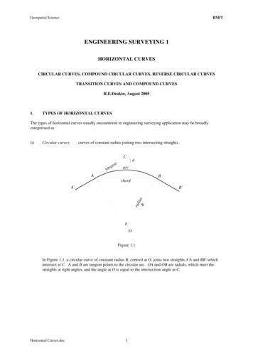
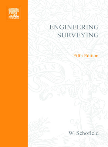
Geospatial ScienceRMITφ s22 LR(5.7)s 2 LRφor(5.8)Note: Since the curvature κ dφ / ds Ks s /( LR ) 1/ ρ , where ρ is the radius of curvature correspondingto the arc s thens ρ LR constant(5.9)This is an important and useful property of the clothoid.When s L (i.e., at the end of the transition curve and the beginning of the circular curve) the total tangentialangle φ L is determined from (5.7) asφL 5.3L2R(5.10)Rectangular coordinates of the clothoid transition curveThe formulae above are not suitable for setting out clothoid transition curves in the field. Instead, rectangularcoordinates of points on the curve will be more useful.In Figure 5.3, P is a point on the clothoid, at a distance s from the start of the curve and the tangent to P cuts thex-axis at an angle φ . The x-y rectangular coordinate system has an origin at A, the start of the transition curve.The x-axis is the extension of the line A'A, i.e., the tangent to the curve at A; the x-coordinate of P is the distancealong the tangent and the y-coordinate is the perpendicular offset from the tangent. A small arc length Δs hascomponents Δx and Δy , and in the limit become infinitesimal changes ds, dx and dy shown in the enlargementto the right.φA'AΔxxsx.yPstart of transitionΔyΔsdx ds cos φφydsdy ds sin φFigure 5.3To express the equation of the clothoid in rectangular coordinates we make use of the differential relationshipsshown in Figure 5.3dx ds cos φdy ds sin φDifferentiating (5.7)dφ sdsLRSubstituting for s using (5.8) and re-arranging givesds Horizontal Curves.docLR dφ2 φ13(5.11)

Geospatial ScienceRMITSubstituting for ds in equations (5.11) and integrating givesx LR φ cos φdφ2 0 φy LR φ sin φdφ2 0 φThese integrals, known as Fresnel integrals cannot be expressed in terms of elementary functions. Instead,cos φ and sin φ are expanded into series and the integration performed term by term with the result expressed asa truncated series, assuming successive terms become smaller and smaller. Thenx LR2y LR2 φ φ00 φ2 2! φ3 3!φ 1/ 2 1 φ 1/ 2 φ φ4 4! φ66!φ5 φ75! 7! φ8 " dφ8! φ9 " d φ9! Performing the integrations and simplifying gives the series expansion for the clothoid in terms of the tangentialangle φ φ2φ4φ6φ8x 2 LR φ 1 " (5)2! (9)4! (13)6! (17)8! (5.12) φ φ3φ5φ7φ9y 2 LR φ " 3 (7)3! (11)5! (15)7! (19)9! (5.13)Substituting for φ from equation (5.7) gives the series expansion for the clothoid in terms of curve length sx s y (s5 s9s13 s17(5 2 ) 2!( LR ) ( 9 2 ) 4!( LR ) (13 2 ) 6!( LR ) (17 2 ) 8!( LR )22446688 "(5.14)s3s7s11s15s19 " 357( 3 21 ) LR ( 7 23 ) 3!( LR ) (11 25 ) 5!( LR ) (15 27 ) 7!( LR ) (19 29 ) 9!( LR )9Note that 5 22) 5 22. Equations (5.14) and (5.15) can be re-arranged into a power series ins2LR2468 s2 s2 s2 s2 1111x s 1 " 5 22 2! LR 9 24 4! LR 13 26 6! LR 17 28 8! LR y (5.15)2468 s2 s2 s2 6 s2 666s 3 1 " 35796 LR 7 2 3! LR 11 2 5! LR 15 2 7! LR 19 2 9! LR (5.16)(5.17)The maximum values of x and y are reached when s L, i.e., at the end of the transition curve. Substituting s L into equations (5.14) (5.15) givesxmax L ymax Horizontal Curves.docL3L5 "240 R 3456 R 4L2L4L6 "36 R 336 R 42240 R 514(5.18)(5.19)

Geospatial Science5.4RMITOffsets from the tangent to the clothoid transition curveFor setting out purposes, it may be desirable to compute the y-coordinate (the offset from the tangent) given thex-coordinate (distance along the tangent). To express y as a function of x, we first obtain s in terms of x by"reversing" the series in x in equation (5.14) using Lagrange's Theorem 1Givens x wF ( s ) or x s wF ( s )(5.20)then2w2 d {F ( x )} f ′ ( x ) 2! dx 3w3 d 2 {F ( x )} f ′ ( x ) 3! dx 2 "f ( s ) f ( x ) wF ( x ) f ′ ( x ) (5.21)nwn d n 1 F xf ′ ( x ) n 1 { ( )} n ! dxwhere f ( s ) is a function of s, f ( x ) and F ( x ) are functions of x, f ′( x ) is the derivative of f ( x ) and w is aconstant.In our case w 1 and we choose f ( s ) s so that f ( x ) x and f ′( x ) 1 givings x F ( x) 1 d1 d n 12n{F ( x )} " {F ( x )}n ! dx n 12! dx(5.22)Now F ( s ) consists of all terms on the right-hand side of (5.14), except the 1st term, noting the change of sign toaccord with x s F ( s ) in equation (5.20)F ( s) s540 ( LR )2 s93456 ( LR )4 "hence F ( x ) is the same series with x replacing sF ( x) x540 ( LR )2 x93456 ( LR )4 "This is the 2nd term in equation (5.22). The 3rd term is obtained as follows{F ( x )}2 2 x14x10x18 " 461600( LR ) 138240( LR ) 11943936( LR )81 d1 10 x 92 "{F ( x )} 2 dx2 1600( LR ) 4 x9 "320( LR ) 41Reversion of a series can be achieved by using Lagrange's Theorem. A proof of this theorem can be found inFormulas and Theorems in Pure Mathematics by George S. Carr (2nd ed, Chelsea Pub. Co., New York, 1970).An application of Lagrange's Theorem can be found in Geodesy and Map Projections, by G.B. Lauf (TAFEPublications, Collingwood, Aust., 1983), where it is used to derive a series expression for the "foot-point"latitude used in conversion of latitudes and longitudes (geodetic coordinates) to Universal Transverse Mercatorprojection coordinates.Horizontal Curves.doc15

Geospatial ScienceRMITThe series in equation (5.22) becomes x5x9x9 " s x " "244 40 ( LR ) 3456 ( LR ) 320 ( LR ) 49 x 9x5 x "2440 ( LR ) 17280 ( LR )(5.23)Substituting this series for s into equation (5.15) gives the series for y in terms of xy 5.5x3x7293x1155397 x15131021x19 "6 LR 105 ( LR )3 237600 ( LR )5 269568000 ( LR )7 7763558400 ( LR )9(5.24)Polar coordinates of the clothoid transition curveFor "setting-out" the clothoid, it may be desirable to determine the polar coordinates of P on the curve.Figure 5.4 shows P having x,y rectangular coordinates. The polar coordinates of P are c, the chord distance andα the "deflection angle" from the tangent (the x-axis).A'φαAxcstart of transition.PxyyFigure 5.4It can be seen from Figure 5.4 thatyx(5.25)xcos α(5.26)tan α and that c x 2 y 2 or preferablyc In practical problems, c and α are calculated from the x and y coordinates computed from the series equationsabove.Horizontal Curves.doc16

Geospatial Science5.6RMITThe shift S of a transition curveTo insert a transition curve between a straight and a circular curve it is necessary to shift the circular curve awayfrom the straight by an amount known as the shift. Similarly in order to insert a transition curve between twocircular curves forming a compound curve it is necessary to move the circular curve with the smaller radiusinwards, or the circular curve with the larger radius outwards.K'.Oρ θS sec 2SK.O'θS tan 2shiftOF.φL. O'Sθ - 2φLθ ρ 2Rρ RDαLESA'sRρ JB rad.MshiftAθφLF GQiuHCθ(R S) tan 2Augmented Tangent LengthFigure 5.5In Figure 5.5, straights A'A and KK' intersect at C. The intersection angle is θ . A circular curve of radius R,centred at O' was originally used to join the two straights, but has been shifted to O to allow for the introductionof two transition curves AB and JK, both of length L. O' has been shifted to O a distance S secθ2where S is theshift, the perpendicular distance EF.From Figure 5.5S BH DE ymax R (1 cos φ L )where ymax is the maximum offset from the tangent given by equation (5.19) and φ L tangential angle (see equation 5.10). Using the expansion cos φ 1 and ymax givesHorizontal Curves.doc17φ22! φ44! φ66!Lis the maximum2R " and substituting for φ L

Geospatial ScienceRMIT L2 L4L6L2L4L6S " R 1 1 2 " 3546 6 R 336 R 42240 R 8R 384 R 46080 R L2 L2 L4L6L4L6 " " 3535 6 R 336 R 42240 R 8R 384 R 46080 R which simplifies toS L2L4L6 "324 R 2688R 506880 R 5(5.27)For many practical applications the shift is approximated byS 5.7L224 R(5.28)The Augmented Tangent Length of a transition curveFrom Figure 5.5, the Augmented Tangent Length is the distance AC whereAC Q FC(5.30)andFC FG GCG is the tangent point of the original circular curve or radius R joining the two straights, GC R tan θ / 2 andFG S tan θ / 2 , hence the Augmented Tangent Length isAC Q ( R S ) tanθ(5.31)2From Figure 5.5Q AH DB xmax R sin φ Lwhere xmax is the maximum distances along the tangent given by equation (5.18) and φ L tangential angle (see equation 5.10). Using the expansion sin φ φ φ33! φ5 φ75! 7!Lis the maximum2R " and substituting for φ Land xmax gives LL3L5L3L5Q L " R " 243540R3456R2R48R3840R LL3L5L3L5 L " " 242440R3456R248R3840R which simplifies toQ LL3L5 "2 240 R 2 34560 R 4(5.32)The Augmented Tangent Length AC becomes L L3L5θAC " ( R S ) tan242 2 240 R 34560 R Horizontal Curves.doc18(5.33)

Geospatial Science5.8RMITClothoid transition curves between circular curvesTwo circular curves of radii R1 and R2 can be joined by a clothoid transition curve whose curvature varies fromκ 1 1/ ρ1 1/ R1 to κ 2 1/ ρ 2 1/ R2 . That is, a transition curve tangential to both circular arcsAρ1 R1φsLφBPxyρ.O1B R2ρ2.O2Figure 5.6Figure 5.6 shows two circular curves of radii R1 and R2 centred at O1 and O2 . A clothoid transition curve ABof length L joins these two circular curves. The curvature of the clothoid at A is κ 1 1/ ρ1 1/ R1 and thecurvature at B is κ 2 1/ ρ 2 1/ R2 and the clothoid has a constant rate of change of curvature with respect to arclength s. Hence, we may link the curvature at P with the curvatures at the beginning and end of the curve byκ P κ1 (κ 2 κ 1 )Ls(5.34)dφ(5.35)The elemental arc length at P isds ρ dφ 1κPSubstituting equation (5.34) and re-arranging gives (κ κ 1 ) dφ κ 1 2s dsL Integrating gives an expression for the tangential angleφ κ 1s κ 2 κ12Lwhere C is a constant of integration.Horizontal Curves.doc19s2 C

Geospatial ScienceRMITSince φ 0 when s 0 then C 0 and the equation for the tangential angle φ becomesφ κ 1s κ 2 κ1s22Ls R R2 2 1sR1 2 LR1 R2and lettingA R1 R22 LR1 R2(5.36)φ s A s2R1(5.37)givesNow similarly to before, the elemental distance ds has components in the x and y directions, where the x,y axeshave an origin at A with the x-axis in the direction of the tangentdx ds cos φdy ds sin φ(5.38)Substituting equation (5.37) for φ in equations (5.38), then expanding using the series expansions for cos φ andsin φ , and then integrating gives246 1 s 1 2 s 1 2 s 2x 1 As As As " dsR1 4! R1 6! R1 0 2! (5.39)357s s 1 s 1 s 1 s y As 2 As 2 As 2 As 2 " dsR1 3! R1 5! R1 7! R1 0 (5.40)sPerforming the integrations and simplifying (using the symbolic mathematical package MAPLE) gives 1 A 4 1A2 5 A 6 A21 7 x s 2 s3 s s s s 43 26 6 R1 4 R1 120 R1 10 36 R1 28R1 5040 R1 A3A 8 A4A2 9 A3 10 ss s 54 3 48R1 960 R1 216 432 R1 360 R1 (5.41) A4 11 A5 12 A6 13 s s s "2 9360 528R1 1440 R1 1 2 A 3 1 4 A 5 1A3 7A2 6 Ay s s s s s s3254 3 2 R1 24 R1 10 R1 720 R1 12 R1 168R1 42 A2 8 A31A 9 A4A2 10 s s s 37265 96 R1 40320 R1 108R1 6480 R1 240 R1 2400 R1 A5A3 11 A4 12 A5 13s s s 4 3 2 1728R1 3120 R1 1320 1584 R1 A6 14 15A7 ss " 2 10080 R1 75600 R1 Horizontal Curves.doc20(5.42)

Geospatial Science5.9RMITPerpendicular Offsets to a Clothoid Transition Curve.yPxoAPφxyoφPota ngentx'yρ RPy'Figure 5.7Certain purposes may require the computation of perpendicular offsets from points of known coordinates to aclothoid transition curve (defined by L and R).Figure 5.7 shows a clothoid transition curve tangential to a straight at A. The extension of the straight is thex-axis and the y-axis is perpendicular to the straight and directed towards the centre of curvature. P is a knownpoint (coordinates xP , y P ) and the perpendicular to the transition curve passing through P intersects the curve atP0 ( x0 , y0 ). The tangent to the curve at P0 intersects the x-axis at an angle φ (the tangential angle). The x'-axisis parallel to the tangent at P0 and the x'-y' axes are rotated from the x-y axes by the angle φ .The method of solution is to first determine the tangential angle φ , and then compute the distance along thecurve between A and P0 using equation (5.8) s 2 LR φ . Having determined the distance s, the x-ycoordinates of P0 can be computed using equations (5.14) and (5.15) and finally the perpendicular offset P0 -Pcomputed from coordinate differences.To determine the tangential angle φ the following formulae and relationships are required.1.The equations of the x-y coordinate of a clothoid transition curve given L and RHorizontal Curves.doc φ2φ4φ6 x 2 LR φ 1 " (5)2! (9)4! (13)6! (5.12) φ φ3φ5φ7 y 2 LR φ " 3 (7)3! (11)5! (15)7! (5.13)21

Geospatial Science2.RMITThe equations for a rotation of coordinate axesx x ′ cos φ y ′ sin φ sin φ x cos φ y (5.43)φx'orx ′ x cos φ y sin φy ′ y cos φ x sin φy'(5.44)yFigure 5.83.Sine and Cosine expansionssin φ φ cos φ 1 φ33!φ22! φ5 φ75!φ44! 7!φ66! "(5.45) "The x' coordinate of any point whose x,y coordinates are known is given by (5.44).x ′ x cos φ y sin φSubstituting the equations for x and y (5.12) and (5.13) and the expansions for sine and cosine (5.45) gives2 φ2φ4φ4 φx ′ 2 LR φ 1 " 1 " ( 5) 2! ( 9 ) 4! 2! 4! φ φ 3 φ 5 φ3φ52 LR φ " φ " 373!115!3!5!( ) ( ) Expanding this equation and then gathering terms gives (1st three terms only) an equation for x' in terms of L, Rand the tangential angle φx ′ 2 LR φ 1 2 4162 LR φ 5 2 2 LR φ 9 215945(5.46)The x' coordinate of P isxP′ xP cos φ y P sin φ φ2 φ4 φ3 φ5 xP 1 " y P φ " 2!4!3!5! Expanding and gathering terms givesxP′ xP y Pφ 1111xPφ 2 y Pφ 3 xPφ 4 y Pφ 52624120(5.47)Now, when x ′ xP′ , the normal to the transition curve will pass through P. Subtracting (5.47) from (5.46) andtaking only terms up to the 3rd power gives2 LR φ 1 2 4112 LR φ 5 2 xP y Pφ xPφ 2 y Pφ 3 01526(5.48)This equation can be solved for φ using Newton's iterative technique. A simplification can be made by usingthe substitutionα φand equation (5.48) can be written asHorizontal Curves.doc22(5.49)

Geospatial ScienceRMITf (α ) 1412 LR α 5 xPα 4 y Pα 2 2 LR α xP 0y Pα 6 6152(5.50)Solving for α φ using Newton's Iterationα n 1 α n f (α n )f ′ (α n )(5.51)where f ′ (α ) is the derivative of f (α ) andf ′ (α ) y Pα 5 42 LR α 4 2 xPα 3 2 y Pα 2 LR3(5.52)A starting value for α can be obtained by substituting α 0 into f (α ) and f ′ (α ) and using (5.51) to giveα1 NOTESxP2 LR(5.53)1. A better (computationally) way to calculate numeric values for f (α ) and f ′ (α ) is to express theequations in a nested form 1 41 2 LR α α xPα α y P α 2 LR α xPf (α ) y Pα α 6 152 4 2 LR α α 2 xPα α 2 y P α 2 LRf ′ (α ) ( y Pα ) α 3 (5.54)2. When using this method to compute perpendicular offsets it should be remembered that thepositive directions of the x and y axes are dictated by the direction of the transition curve. Theymay be opposite to the positive directions of East and North coordinate axes. Hence, care shouldbe taken when determining xP and y P from E,N coordinates.Horizontal Curves.doc23

Geospatial Science5.9RMITFitting a Clothoid Spiral Transition Curve Between a Straight and a Circular CurveAXTSRcosφdRLtransitionφLcur veOxmaxRcirculararcφLSCymaxA'Figure 5.9In Figure 5.9 a circular curve of radius R has a fixed centre at O having known coordinates. AA' is a straight ofknown bearing and it is desired to find the length L of a clothoid spiral transition curve that is tangential to thestraight at TS and the circular curve at SC. The locations of SC and TS are unknown. X is a point on the straightAA' of known coordinates and the bearing and distance OX can be computed and then the perpendicular distanced from the centre O to the straight. The distance d must be greater than the radius R. From the diagram it can beseen that the spiral angle φ L L ( 2 R ) (which is unknown) is also the angle at the centre O between the radial toSC and the perpendicular to the straight. The distance d is given by L d R cos φ L ymax R cos ymax 2R With the use of an Excel spreadsheet for computing clothoid spirals given parameters L and R, the length of thetransition curve L can be determined by successively changing L, until the required distance d is obtained.φ L L ( 2 R ) can be computed and the radial bearing to SC determined.Horizontal Curves.doc24

Geospatial Science6.RMITDESIGN CONSIDERATIONS FOR CIRCULAR CURVES AND TRANSITIONCURVESCircular curves and transition curves (clothoids) are uniquely defined if any two of their "properties" (orparameters) are fixed. For circular curves these two properties are usually selected from the following: radius,arc length, intersection angle, tangent length or chord length. For transition curves the properties are selectedfrom minimum radius, length of curve, maximum tangential angle (also known as spiral angle) and shift.Generally, in practical design of roads and railways, intersection angles of straight sections are predetermined bythe overall layout and the problem is to design the connecting circular curves and transition curves to suit theexpected traffic conditions. From a traffic viewpoint, the largest possible circular curves and the longestpossible tra

Geospatial Science RMIT (ii) Compound circular curves: two or more consecutive circular curves of different radii. A B C O O 1 2 R RR R R R 1 11 2 2 2 θ θ 12 θ θ θ 1 2 D A' B' Figure 1.2 In Figure 1.2, a compound circular curve ADB joins two straights A'A and BB' which intersect at C.A and B are tangent points to circular arcs of radii R1 and R2 respectively.