WIXLIB

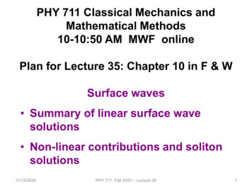
PHY 711 Classical Mechanics andMathematical Methods10-10:50 AM MWF onlinePlan for Lecture 35: Chapter 10 in F & WSurface waves Summary of linear surface wavesolutions Non-linear contributions and solitonsolutions11/13/2020PHY 711 Fall 2020 -- Lecture 351

This material is covered in Chapter 10 ofyour textbook using similar notation.11/13/2020PHY 711 Fall 2020 -- Lecture 352

11/13/2020PHY 711 Fall 2020 -- Lecture 353

Schedule for weekly one-on-one meetings(EST)Nick – 11 AM MondayTim – 9 AM TuesdayGao – 9 PM TuesdayJeanette – 11 AM FridayDerek – 12 PM Friday11/13/2020PHY 711 Fall 2020 -- Lecture 354

Your questions –From Gao –1. In what situation, the velocity potential phi in Bernoulli's equation satisfiesd(phi)/d(t) 0？2. In visualization, what do the red line and the blue line stand for?3. Why does zero vertical velocity at the bottom of a pool ensure all oddderivatives vanish from the Taylor expansion?From Nick –11/13/2020PHY 711 Fall 2020 -- Lecture 355

Consider a container of water with average height h andsurface h ζ(x,y,t)Atmospheric pressure p0 is in equilibrium at the surfacep0ζzhyx11/13/2020PHY 711 Fall 2020 -- Lecture 356

p0ζzhyxEuler's equation for incompressible fluid: p pdvFor irrotational flow -- v Φ U f applied dtρρ Φp g ( z h) 0Linearized equation: Continuity equation within the fluidρ t ρp0 Φ ( ρ v ) 0 v 0 gζ 0At surface: z h ζ t tρ11/13/2020PHY 711 Fall 2020 -- Lecture 357

Keep only linear terms and assume that horizontal variation isonly along x: 2 2 For 0 z h ζ : Φ 2 2 Φ ( x, z ,t) 0 x zConsider and periodic waveform: Φ ( x , z , t ) Z ( z ) cos ( k ( x ct ) )2 d2 2 k 2 Z ( z) 0 dz Boundary condition at bottom of tank: vz ( x,0, t ) 0 dZ0Z ( z ) A cosh(kz )(0) dzAt surface:Also: Φ ( x, h ζ , t ) ζz h ζ vz ( x, h ζ , t ) t z Φ ( x, h ζ , t )p0 gζ 0 tρ 2 Φ ( x, h ζ , t ) 2 Φ ( x, h ζ , t ) Φ ( x, h ζ , t ) ζ g g 022 t t z t11/13/2020PHY 711 Fall 2020 -- Lecture 358

Velocity potential: Φ ( x, z , t ) A cosh(kz ) cos ( k ( x ct ) )At surface:Φ ( x, ( h ζ ) , t ) A cosh(k ( h ζ )) cos ( k ( x ct ) ) 2 2sinh(k ( h ζ )) A cosh(k ( h ζ )) cos ( k ( x ct ) ) k c gk0 cosh(k ( h ζ )) g sinh(k ( h ζ )) g2 c tanh(kh)k cosh(k ( h ζ )) kNote that this solution represents a pure plane wave. Morelikely, there would be a linear combination of wavevectors k.Additionally, your text considers the effects of surfacetension. In this lecture, we will focus on the effects of thenon-linear effects of Euler and continuity equations.11/13/2020PHY 711 Fall 2020 -- Lecture 359

Surface waves in an incompressible fluidGeneral problemincludingp0non-linearitiesζhzyxWithin fluid:0 z h ζ Φ 1 2constant 2 v g ( z h) t 2Φ 0 At surface:z h ζΦ Φ ( x, y, z , t )v v ( x, y, z , t ) Φ ( x, y, z , t )ζ ( x, y , t )with ζ dζ ζ ζ ζ Φ ( x, y, z , t ) vx vy zdt t x y11/13/2020z h ζPHY 711 Fall 2020 -- Lecture 35where vx , y v x , y ( x, y , h ζ , t )10

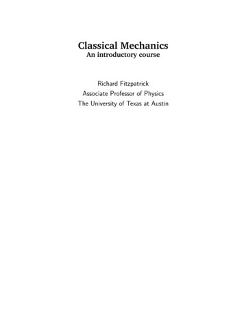
Your question – why is the following true?At surface:z h ζζ ( x, y , t )with ζ dζ ζ ζ ζ Φ ( x, y, z , t ) vx vy dt t x y zz v x , y ( x, y , h ζ , t )where vx , y h ζdζNote that vz ( x, y, h ζ , t ) dtFrom wikipedia11/13/2020PHY 711 Fall 2020 -- Lecture 3511

Your question -- In what situation, the velocity potential phi inBernoulli's equation satisfies d(phi)/d(t) 0?Within fluid:0 z h ζ Φ 1 2 2 v g ( z h) Φ Φ ( x, y , z , t )constant t 2Φ 0 v v ( x, y, z , t ) Φ ( x, y, z , t ) ΦOne example of 0 would be for v 2 0 and z h. t11/13/2020PHY 711 Fall 2020 -- Lecture 3512

p0ζhzyxFurther simplifications; assume trivial y - dependenceζ ζ ( x, t )Φ Φ ( x, z , t )Within fluid :0 z h ζ Φ dζAt surface : v z ( x, z h ζ , t ) zdt11/13/2020PHY 711 Fall 2020 -- Lecture 3513

Non-linear effects in surface waves:p0ζhz 0zyxDominant non-linear effects soliton solutions 3η0 x ct ζ ( x, t ) η0 sech h 2h 2where c11/13/2020η0 constant η0 gh 1 1 η0 / h2h ghPHY 711 Fall 2020 -- Lecture 3514

Detailed analysis of non-linear surface waves[Note that these derivations follow Alexander L. Fetter andJohn Dirk Walecka, Theoretical Mechanics of Particles andContinua (McGraw Hill, 1980), Chapt. 10.]We assume that we have an incompressible fluid: ρ constantVelocity potential: Φ ( x, z , t ); v ( x, z , t ) Φ ( x, z , t )The surface of the fluid is described by z h ζ(x,t). It isassumed that the fluid is contained in a structure(lake, river, swimming pool, etc.) with a structurelessbottom defined by the z 0 plane and filled to anequilibrium height of z h.11/13/2020PHY 711 Fall 2020 -- Lecture 3515

Defining equations for Φ(x,z,t) and ζ(x,t)where 0 z h ζ ( x, t )Continuity equation:v 0 2 Φ ( x, z , t ) 2 Φ ( x, z , t ) 022 x zBernoulli equation (assuming irrotational flow) and gravitationpotential energy22 Φ ( x, z , t ) 1 Φ ( x, z , t ) Φ ( x, z , t ) 0. g ( z h) t2 x z 22xzv11/13/2020vPHY 711 Fall 2020 -- Lecture 3516

Boundary conditions on functions –Zero velocity at bottom of tank: Φ ( x,0, t ) 0. zConsistent vertical velocity at water surface ζdζ v ζ v z ( x , z , t ) z h ζ tdt ζ ζ vx x t Φ ( x, z , t ) Φ ( x, z , t ) ζ ( x, t ) ζ ( x, t ) z x x t11/13/2020PHY 711 Fall 2020 -- Lecture 35 0z h ζ17

Analysis assuming water height z is small relative tovariations in the direction of wave motion (x)Taylor’s expansion about z 0:z 2 2Φz 3 3Φz 4 4Φ Φ( x,0, t ) ( x,0, t ) ( x,0, t ) ( x,0, t ) Φ ( x, z , t ) Φ ( x,0, t ) z2342 z3! z4! z zNote that the zero vertical velocity at the bottom suggestthat to a good approximation, that all odd derivatives nΦvanish from the Taylor expansion. In addition,(x,0,t) z nthe Laplace equation allows us to convert all evenderivatives with respect to z to derivatives with respect to x.z 2 2Φz 3 3Φz 4 4Φ Φ( x,0, t ) ( x,0, t ) ( x,0, t ) ( x,0, t ) Φ ( x, z , t ) Φ ( x,0, t ) z2342 z3! z4! z z 2 Φ ( x, z , t ) 2 Φ ( x, z , t ) 022 x zz 2 2Φz 4 4ΦModified Taylor′s expansion: Φ ( x, z , t ) Φ ( x,0, t ) ( x,0, t ) ( x,0, t ) 242 x4! x11/13/2020PHY 711 Fall 2020 -- Lecture 3518

Question -- Why does zero vertical velocity at the bottom of apool ensure all odd derivatives vanish from the Taylorexpansion?Comment – You are right it is not a rigorous, but anapproximate result.Φ ( x, z , t ) A cosh(kz ) cos ( k ( x ct ) )Example from linear case: n Φ ( x, z , t ) 0In this case all odd derivativesn zz 0One can think of other counter examples of functions forwhich the first derivative vanishes but the third derivativedoes not.11/13/2020PHY 711 Fall 2020 -- Lecture 3519

Check linearized equations and their solutions:Bernoulli equations -Bernoulli equation evaluated at z h ζ ( x, t ) Φ ( x, h, t )0 gζ ( x, t ) tConsistent vertical velocity at z h ζ ( x, t ) Φ ( x, z , t ) ζ ( x, t ) z t 0z h ζUsing Taylor's expansion results to lowest order Φ ( x, h, t ) 2Φ ( x,0, t ) ζ ( x, t ) h z x 2 tDecoupled equations: Φ ( x, h, t ) Φ ( x,0, t ) gζ ( x, t ) t t 2Φ ( x,0, t ) 2Φ ( x,0, t ). gh22 t x linear wave equation with c2 gh11/13/2020PHY 711 Fall 2020 -- Lecture 3520

Analysis of non-linear equations -Bernoulli equation evaluated at surface:22 Φ ( x, z , t ) 1 Φ ( x, z , t ) Φ ( x, z , t ) t x z2 gζ ( x, t ) 0.z h ζConsistency of surface velocity Φ ( x, z , t ) Φ ( x, z , t ) ζ ( x, t ) ζ ( x, t ) z x x t 0z h ζRepresentation of velocity potential from Taylor′s expansion:z 2 2Φz 4 4ΦΦ ( x, z , t ) Φ ( x,0, t ) ( x,0, t ) ( x,0, t ) 242 x4! x11/13/2020PHY 711 Fall 2020 -- Lecture 3521

Analysis of non-linear equations -- keeping the lowestorder nonlinear terms and include up to 4th orderderivatives in the linear terms. Let φ ( x, t ) Φ ( x,0, t )Approximate form of Bernoulli equation evaluated at surface: z h ζ222 1 φ φ (h ζ ) φ φ (h ζ ) 2 gζ 02 t t x x 22 x 232 φ h 2 3φ1 φ gζ 0.2 t2 t x2 x Approximate form of surface velocity expression : φ h3 4φ ζ (h ζ ( x, t )) 0.4 x x 3! x tThese equations represent non-linear coupling of φ ( x, t ) and ζ ( x, t ).11/13/2020PHY 711 Fall 2020 -- Lecture 3522

21 φ φ h 2 3φ Coupled equations: 0. gζ 2 t2 t x2 x φ h3 4φ ζ 0. (h ζ ( x, t )) 4 x x 3! x tTraveling wave solutions with new notation:φ ( x, t ) χ (u )u x ctand ζ ( x, t ) η (u )Note that the wave “speed” c will be consistentlydetermined2d χ (u ) ch d χ (u ) 1 d χ (u ) 0.c gη (u ) 32 du2 du du23d d χ (u ) h3 d 4 χ (u )dη (u ) c 0. (h η (u )) 4du du 6 dudu11/13/2020PHY 711 Fall 2020 -- Lecture 3523

Integrating and re-arranging coupled equations223d χ (u ) ch d χ (u ) 1 d χ (u ) 0.c gη (u ) 32 du2 du du221gh2ghgg η χ ''' ( χ ') 2 η χ' η '' 3 η 222c2c2cccd d χ (u ) h3 d 4 χ (u )dη (u ) c 0. (h η (u )) 4du du 6 dudud χ (u ) h3 d 3 χ (u ) (h η ) cη (u ) 036 dudud χ (u )Now we can express χ ′ in terms of η :dugh2 gg2 2χ′ η η '' 3 ηc2c2c11/13/2020PHY 711 Fall 2020 -- Lecture 3524

Integrating and re-arranging coupled equations – continued -Expressing modified surface velocity equation in terms of η(u):223 g h gg 2hg(h η ) η 0η '' 3 η η '' cη 2c2c c 6c3ghghg gh 2 1 2 η 2 η '' 2 1 2 η 03cc c 2c 23h2 hg 1 2 η (u ) η ''(u ) [η (u ) ] 0.32hc 2Note: c gh 11/13/2020PHY 711 Fall 2020 -- Lecture 3525

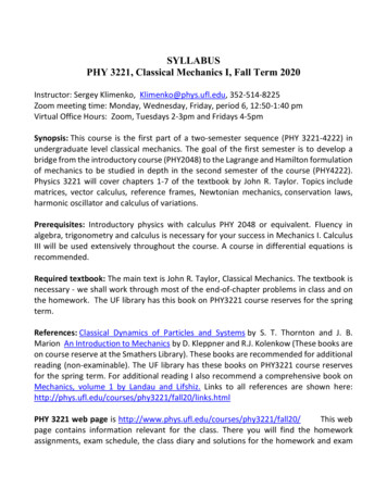
Solution of the famous Korteweg-de Vries equationModified surface amplitude equation in terms of η3h22 hg 1 2 η (u ) η ''(u ) [η (u ) ] 0.32hc Soliton solution 3η0 x ct ζ ( x, t ) η ( x ct ) η0 sech hh2 2 c11/13/2020 η0 gh 1 h1 η0 / h2 ghwhere η0 is a constantPHY 711 Fall 2020 -- Lecture 3526

Steps to solution3h22 hg ηηη1()''()()0.uuu[ ] 2 32hc η03hg η0h22 η (u ) η ''(u ) [η (u ) ] Let 1 2 0.32hchh1 3 d η0 2h2 2 Multiply equation by η '(u )0 η (u ) η ' (u ) η (u ) 62hdu 2h Integrate wrt u and assume solution vanishes for u η01 3h2 2η (u ) η ' (u ) η (u ) 02h62h3 22η ' (u ) 3 η (u ) (η0 η (u ) )hη03dη η (u ) du1/ 23h 3η0 η (η0 η )2cosh u3 4h 211/13/2020PHY 711 Fall 2020 -- Lecture 3527

3η0 x ct ζ ( x, t ) η ( x ct ) η0 sech h 2h 211/13/2020PHY 711 Fall 2020 -- Lecture 3528

Your question -- In visualization, what do the red line andthe blue line stand for?Two soliton solutions with different amplitudes11/13/2020PHY 711 Fall 2020 -- Lecture 3529

Relationship to “standard” form of Korteweg-de Vries equationNew variables: β 2 η0 , x3 x,2h h andt3 ct.2h 2η0 hStandard Korteweg-de Vries equation η η 3η0. 6η 3 t x xSoliton solution:η(x, t )11/13/2020 β sech ( x β t ) .2 2 β2PHY 711 Fall 2020 -- Lecture 3530

More detailsModified surface amplitude equation in terms of η :23hgh2 ′′0. 1 2 η (u ) η (u ) [η (u ) ] 32hc η η dηgh ηdη c ; Some identities: 0 1 2 ;. t x duhcduDerivative of surface amplitude equation:η03h20.η ' η ''' ηη ' 3hhExpression in terms of x and t:η0 ηh 2 3η 3 η η 0.3ch th x3 xExpression in terms of x and t : η η 3η0. 6η 3 t x x11/13/2020PHY 711 Fall 2020 -- Lecture 3531

SummarySoliton solution 3η0 x ct ζ ( x, t ) η ( x ct ) η0 sech h 2h 2 c11/13/2020 η0 gh 1 1 η0 / h 2h ghwhere η0 is a constantPHY 711 Fall 2020 -- Lecture 3532

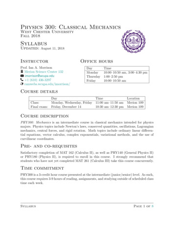
Photo of canal soliton http://www.ma.hw.ac.uk/solitons/Some links:Website – http://www.ma.hw.ac.uk/solitons/11/13/2020PHY 711 Fall 2020 -- Lecture 3533

https://www.macs.hw.ac.uk/ chris/scott russell.html11/13/2020PHY 711 Fall 2020 -- Lecture 3534

PHY 711 Classical Mechanics and Mathematical Methods . Non-linear contributions and soliton solutions. 11/13/2020 PHY 711 Fall 2020 -- Lecture 35 2 This material is covered in Chapter 10 of your textbook using similar notation. 11/13/2020 PHY 711 Fall 2020 -- Lecture 35 3. . derivatives vanish from the Taylor expansion?