Transcription
Computing Higher Order Derivatives of Matrix andTensor ExpressionsSören LaueFriedrich-Schiller-Universität JenaGermanysoeren.laue@uni-jena.deMatthias MitterreiterFriedrich-Schiller-Universität m GiesenFriedrich-Schiller-Universität ization is an integral part of most machine learning systems and most numerical optimization schemes rely on the computation of derivatives. Therefore,frameworks for computing derivatives are an active area of machine learning research. Surprisingly, as of yet, no existing framework is capable of computinghigher order matrix and tensor derivatives directly. Here, we close this fundamentalgap and present an algorithmic framework for computing matrix and tensor derivatives that extends seamlessly to higher order derivatives. The framework can beused for symbolic as well as for forward and reverse mode automatic differentiation.Experiments show a speedup of up to two orders of magnitude over state-of-the-artframeworks when evaluating higher order derivatives on CPUs and a speedup ofabout three orders of magnitude on GPUs.1IntroductionRecently, automatic differentiation has become popular in the machine learning community due to itsgenericity, flexibility, and efficiency. Automatic differentiation lies at the core of most deep learningframeworks and has made deep learning widely accessible. In principle, automatic differentiationcan be used for differentiating any code. In practice, however, it is primarily targeted at scalarvalued functions. Current algorithms and implementations do not produce very efficient code whencomputing Jacobians or Hessians that, for instance, arise in the context of constrained optimizationproblems. A simple yet instructive example is the function f (x) x Ax, where A is a square matrixand x is a vector. The second order derivative of this function, i.e., its Hessian, is the matrix A A.Frameworks like TensorFlow [1], Theano [23], PyTorch [16], or HIPS autograd [14] generate code forthe second order derivative of f that runs two to three orders of magnitude slower than the evaluationof the expression A A.In machine learning, automatic differentiation is mostly used for numerical optimization. Manymachine learning optimization problems are formulated in standard matrix language. This has notonly the advantage of a compact problem representation, but linear algebra expressions can also beexecuted efficiently on modern CPUs and GPUs by mapping them onto highly tuned BLAS (basiclinear algebra subprograms) implementations that make extensive use of vectorization such as theSSE and the AVX instruction sets or SIMD architectures. Ideally, these advantages are kept alsofor the gradients and Hessians of the expressions that encode the optimization problem. This is thepurpose of matrix calculus that computes, if possible, derivatives of matrix expressions again as32nd Conference on Neural Information Processing Systems (NIPS 2018), Montréal, Canada.
matrix expressions. In matrix calculus, the gradient of f (x) x Ax is the expression A x Axand its Hessian is the expression A A, which can be efficiently evaluated.Surprisingly, none of the classic computer algebra systems such as Mathematica, Maple, Sage, orSymPy1 supports matrix calculus. These systems calculate derivatives of a given matrix expressiononly on matrix entry level, i.e., every matrix entry gives rise to a separate symbolic scalar variable.Each of these systems is able to compute derivatives of univariate scalar-valued functions. Hence,while in pure matrix calculus a matrix A Rn n is represented by just one variable, the classiccomputer algebra systems treat this as n2 variables. Thus, the number of input variables increasesdramatically and the complexity of evaluating derivatives explodes. Also, it is impossible to read offthe derivative in matrix notation from such complex expressions. These drawbacks are also present inthe classic frameworks for automatic differentiation that mostly compute derivatives only on scalarlevel, like ADOL-C [25] or TAPENADE [10]. While the direct integration of matrix and tensoroperators into automatic differentiation frameworks like TensorFlow is under active development, sofar the output functions still have to be scalar. Hence, higher order derivatives or Jacobians cannot becomputed directly.Contributions. We provide an algorithmic framework for computing higher order derivatives ofmatrix and tensor expressions efficiently, which fully operates on tensors, i.e., all variables areallowed to be tensors of any order, including the output variables. Therefore, for the first time higherorder derivatives and Jacobians can be computed directly. The derivatives are represented as compactmatrix and tensor expressions which can be mapped to efficient BLAS implementations. Other stateof-the-art frameworks produce huge expression graphs when deriving higher order derivatives. Theseexpression graphs cannot be mapped to simple BLAS calls but involve many for-loops and complexmemory access. Hence, we observe an increase in efficiency of up to two orders of magnitude onCPUs. Since GPUs can deal with this even worse we observe here an increase in efficiency of aboutthree orders of magnitude over current state-of-the-art approaches. An important benefit of workingon tensors is that it enables symbolic matrix calculus. We show that the predominantly used standardmatrix language is not well suited for symbolic matrix calculus, in contrast to a tensor representation.Thus, to implement matrix calculus, we first translate linear algebra matrix expressions into a tensorrepresentation, then compute derivatives in this representation and finally translate the result backinto the standard matrix language.Related work. A great overview and many details on fundamentals and more advanced topics ofautomatic differentiation can be found in the book by Griewank and Walther [9]. Baydin et al. [2]provide an excellent survey on the automatic differentiation methods used within machine learning.Pearlmutter [17] discusses the following approach for computing higher order derivatives, like theHessian of a function f : Rn R, by automatic differentiation: First, an expression for the gradient f is computed. Then the Hessian is computed column-wise by multiplying the gradient with thestandard basis vectors ei , i 1, . . . , n and differentiating the resulting n scalar functions ( f ) ei .The derivative of ( f ) ei gives the i-th column of the Hessian of f . Gebremedhin et al. [7] showthat a few columns of the Hessian can be computed at once with help of graph coloring algorithms, ifthe Hessian is sparse and has a special structure. However, if the Hessian has no special structure,then all n columns need to be computed individually. This can be seen, for instance, in TensorFlow’sexpression graph for computing the Hessian of x Ax that has more than one million nodes for a stillreasonably small value of n 1000.An alternative approach is presented in the book by Magnus and Neudecker [15] that provides anextensive number of rules for deriving matrix derivatives. At its core, matrices are turned into vectorsby the vec function that stacks the columns of a matrix into one long vector. Then the Kroneckermatrix product is used to emulate higher order tensors. This approach works well for computing firstorder derivatives. However, it is not practicable for computing higher order derivatives. Also, manyof the rules rely on the fact that the vec function assumes column-major ordering (Fortran style). Ifhowever, one switches to a programming language that uses row-major ordering (C style), then someof the formulas do not hold anymore. For instance, the Python NumPy package that is widely used inthe machine learning community follows row-major ordering when used with standard settings. Tobe independent of such a convention and to be able to compute higher order derivatives, we workdirectly with higher order tensors.1Earlier versions of SymPy contained an algorithm for computing matrix derivatives. However, since it sometimes produced erroneous results it has been removed, see, e.g., https://github.com/sympy/sympy/issues/10509.2
The work by Giles [8] collects a number of derivatives for matrix operators, i.e., pushforwardand pullback functions for automatic differentiation. Similarly, Seeger et al. [22] provide methodsand code for computing derivatives for Cholesky factorization, QR decomposition, and symmetriceigenvalue decomposition when seen as matrix operators. However, they all require that the outputfunction is scalar-valued, and hence, cannot be generalized to higher order derivatives.2Languages for matrix and tensor expressionsMatrix expressions are typically written in a simple yet very effective language. This languagefeatures two types of entities, namely objects and operators. The objects of the language are scalars,vectors and matrices, and the operators include addition, various forms of multiplication, transposition,inverses, determinants, traces, and element-wise functions that can be applied to objects.Problems with the standard matrix language. Since matrices can be used to encode differententities like linear maps, bilinear maps, and transformations that describe a change of basis, the matrixlanguage sometimes enforces an indirect encoding of these entities. For instance, let the squarematrix A encode a bilinear map on some vector space, i.e., the entries of A represent the evaluation ofthe bilinear map on any combination of basis vectors. Assume we want to evaluate the bilinear mapat the vectors x and y whose entries store the respective coefficients with respect to the same basisthat is used for specifying A. The evaluation of the bilinear map at x and y is then typically written asx Ay, which basically means: apply the linear map that is encoded by A to y and feed the resultingvector into the linear form x . Note that transposing a vector means mapping it to an element inthe dual vector space. The scalar value x Ay is not affected by the change of interpretation; thevalue of the bilinear map evaluated at x and y is the same as the value of the evaluation of the linearform x at the vector Ay. Hence, the existence of different interpretations is not a problem whenevaluating matrix expressions. But it becomes a problem once we want to compute derivatives ofsuch expressions. For instance, if we want to compute the derivative of the expression x Ax withrespect to the vector x, then we also need to compute the derivative of the transformation that maps xinto the linear form x , and it is not obvious how to do this. In fact, matrix notation does not containan expression to represent this derivative.Ricci calculus. The problem is avoided by turning to a different language for encoding matrixexpressions, namely Ricci calculus [20]. Ricci calculus lacks the simplicity of the standard languagefor matrix expressions, but is more precise and can distinguish between linear maps and bilinear mapsthrough the use of indices. In Ricci calculus one distinguishes two types of indices, namely upper(contravariant) and lower (covariant) indices, that determine the behavior of the encoded objects underbasis changes. Scalars have no index, vectors have one upper, and covectors one lower index. Bilinearforms on a vector space have two lower indices, bilinear maps on the dual space have two upperindices, and linear maps have one upper and one lower index. Hence, the bilinear map A evaluated atthe vectors x and y is written in Ricci calculus as xi Aij y j , or equivalently Aij xi y j . Ricci calculusdoes not include the transposition transformation, but features δ-tensors. The linear identity mapis encoded in Ricci calculus by the δ-tensor δji . The δ-tensors δij and δ ij have no interpretation aslinear maps but serve the purpose of transposition; a vector xi is mapped by δij to the covector δij xiand the covector xi is mapped by δ ij to the vector δ ij xi . In Ricci calculus one distinguishes betweenfree and bound indices. Bound indices appear as lower and also as upper indices in the expression,while free indices appear either as lower or upper indices. Hence, the expression δij xi has one free,lower index, namely j, and thus encodes a covector, while δ ij xi has one free, upper index, again j,and encodes a vector. The expression Aij xi xj has no free indices and thus encodes a scalar.Let us come back to the issue of the interpretation of an expression. The different interpretations of theexpression x Ay can be distinguished in Ricci calculus; Aij xi y j is a bilinear map evaluated at thevectors xi and y j , and xi Aij y j is the linear form xi evaluated at the vector Aij y j . The interpretationthat the vector x is first mapped to the covector x and then evaluated at the image of the vector yafter applying the linear map A is written in Ricci calculus as xi δij Ajk y k .Hence, our approach for computing derivatives of matrix expressions is to translate them first intoexpressions in Ricci calculus, see Table 1 for examples, and then to compute the derivatives for theseexpressions. The resulting derivative is again an expression in Ricci calculus that can be translatedback into the standard matrix calculus language.3
Table 1: Translation of expressions from matrix notation into the Ricci calculus language. Here,denotes the element-wise multiplication and diag(x) the matrix whose diagonal is the vector x.Matrix notationRicci calculusMatrix notationRicci calculusc x yx Ayx y AC A·Bc xi y ixi Aij y jxj yi AijCki Aij BkjA xy z x yB A diag(x)B diag(x)AAij xi yjz i xi y iBji Aij xjBji xi AijElements of Ricci calculus. Only objects with exactly the same indices can be added or subtracted.For instance, the addition xi y i is a valid expression in Ricci calculus, but the expression xi y j isnot. Obviously, also xi xi is not a valid expression, because there is no addition of vectors andcovectors. The standard multiplication of objects that do not share an index is the outer product (orstandard tensor product). For example, the product xi yj describes a matrix that encodes a linear map.A multiplication that contains the same index once as an upper and once as a lower index describesan inner product, or contraction. A contraction entails the sum over all entries in the object that areaddressed by the shared index. For instance, xi yi encodes the evaluation of the linear form yi at thevector xi , Aji xi encodes the evaluation of the linear map Aji at the vector xi . Note that, in contrast tostandard matrix multiplication, multiplication in Ricci calculus is commutative. This will be veryhelpful later when we are deriving algorithms for computing derivatives. Applying element-wiseunary functions like exp to some object keeps the indices, i.e., exp(Aij ) exp(A)ij .Our version of Ricci calculus also features some special symbols. For instance, 0ij encodes the linearmap that maps any vector to 0. Hence, all entries of the matrix 0ij are 0. Similarly, 0i encodes the0-vector. The determinant of a matrix Aji is denoted as det(Aji ). The trace of Aji does not need aspecial symbol in Ricci calculus, because it can be encoded by the expression Aji δji .Extension to higher order tensors. Since Ricci calculus can be extended easily to include moregeneral tensor expressions we can also generalize our approach to computing gradients of moregeneral tensor expressions. Higher order tensors just have more (free) indices. Note that for encodinghigher order tensors, the use of some form of indices is unavoidable. Hence, we can use the Riccicalculus language directly for specifying such expressions and their derivatives; there is no need fortranslating them into another language. However, the translation makes sense for matrix expressionssince the succinct, index free, standard language is very popular and heavily used in machine learning.3Tensor calculusTo process mathematical expressions, we usually represent them by a tree, or more generally, by adirected acyclic graph (DAG). The roots of the DAG, referred to as input nodes, have no parents andrepresent the variables. The leaves of the DAG, or output nodes, have no children and represent thefunctions that the DAG computes. Let the DAG have n input nodes (variables) and m output nodes(functions). We label the input nodes x[0], ., x[n 1], the output nodes y[0], ., y[m 1], and theinternal nodes v[0], . . . , v[k 1]. Every internal and every output node represents either a unary or abinary operator. The arguments of these operators are supplied by their parent nodes. Hence, everynode in the DAG can have at most two parents, but multiple children. Every edge that connects aparent x with a child f is labeled by the easy to compute derivative of f with respect to x, i.e., thederivative f x . For instance, if f x · y (multiplication operator), then the label of the edge (x, f ) isy. In case of f x y (addition operator), the label of this edge would be 1, and for f sin(x)(sine operator), the label is cos(x). Figure 1 illustrates the case f x Ax.In automatic differentiation, one distinguishes between forward and reverse mode. Both modes arederived from the chain rule. In forward mode, the derivative of the roots is computed from roots toleaves along the edges and in reverse mode they are computed from leaves to roots. The edge labelsare then multiplied along all paths and the products are summed up and stored in the nodes of theDAG.4
Forward mode. In forward mode for computing derivatives with respect to the input variable x[j], v[i]each node v[i] will eventually store the derivative v̇[i] x[j], that is computed from root to leaves: x[i]At the root nodes representing the variables x[i], the derivatives x[j]are stored. Then the derivativesthat are stored at the remaining nodes, here called f , are iteratively computed by summing over alltheir incoming edges using the following equation:XX f f x ff · ẋ,(1) x[j] x x[j] xx : x is parent of fx : x is parent of f f xwhere theare the labels of the incoming edges of f and the ẋ have been computed before andare stored at the parent nodes x of f . This means, the derivative of each function is stored at thecorresponding leaves y[i] of the expression DAG. Obviously, the updates can be done simultaneouslyfor one input variable x[j] and all output nodes y[i]. Computing the derivatives with respect to allinput variables requires n such rounds.Reverse mode. Reverse mode automatic differentiation proceeds similarly, but from leaf to roots.Each node v[i] will eventually store the derivative v̄[i] y[j] v[i] , where y[j] is the function to bedifferentiated. This is done as follows: First, the derivatives y[j] y[i] are stored at the leaves of the DAG.Then the derivatives that are stored at the remaining nodes, here called x, are iteratively computed bysumming over all their outgoing edges using the following equation:XX y[j] f f y[j] · f ·,(2)x̄ x f x xf : f is child of xf : f is child of xwhere theare the labels of the outgoing edges of x and the f have been computed before andare stored at the children f of x. This means, that the derivative of the function y[j] with respectto all the variables x[i] is stored at the corresponding roots of the expression DAG. Computing thederivatives for all the output functions requires m such rounds. f xTensor calculus. Tensor calculus can be implemented straightforwardly using either the forward orreverse mode. The input nodes are now considered tensors (symbols) like xi or Aii . These symbolsare combined by the inner and the output nodes of the expression DAG into more complex tensorexpressions like Aji xi . In contrast to existing approaches, the output nodes can represent non-scalartensor expressions, too. To compute the derivatives, the edges of the expression DAG are labeledby the corresponding tensor derivatives v̇[i] in forward mode and v̄[i] in reverse mode, respectively.Derivatives are then computed at expression level as described above. To the best of our knowledge,this is the first approach for applying automatic differentiation to matrix and tensor expressions thattreats forward and reverse mode equally. We show in Section 4 that the symbolic expressions forhigher order derivatives, obtained through this approach, can be evaluated very efficiently.Why is standard matrix calculus more complicated? The standard language for matrix expressionsin linear algebra is, as discussed in Section 2, not precise. The multiplication operator, in particular, isoverloaded and does not refer to one but to several different multiplications. The following examplesillustrate how this lack of precision complicates the process of computing derivatives.Consider the simple matrix multiplication C AB as part of an expression DAG. It holds, thatĊ ȦB AḂ for the forward mode and Ā C̄B and B̄ A C̄ for the reverse mode, see [8].These equations cannot be instantiations of Equations (1) and (2) for the following reasons: Considerthe two edges from the (parent) nodes that represent A and B, respectively, to the node that represents CC AB. We have C A B and B A. In forward mode we have to multiply the differential Ȧ Cwith C A from the right and the differential Ḃ with B from the left. In Equation (1), though, bothmultiplications are always from the left. Similarly, in reverse mode, we also multiply once from theleft and once from the right, while both multiplications are always from the right in Equation (2). CFurthermore, the multiplication in reverse mode is not with C A and B , respectively, but with theirtransposes. This might seem negligible at first, to be fixed by slight adjustments to Equations (1)and (2). The expression c det(A) shows that this is not so easy. The DAG for this expressionhas only two nodes, an input node (parent) that represents the matrix A and its child (output node)that represents c det(A). In forward mode, conventional approaches yield ċ c tr(inv(A)Ȧ),yet Ā c̄c inv(A) in reverse mode, see again [8]. It is impossible to bring these equations into5
y[0]y[0]1x[0]v[2]x[1]v[1] v[3] v[1]Akjv[1]x[1] 1v[4]x[0]Aijv[0]v[2]δikδiix[1] Aijxiv[2]δjix[0]v[2] δ jk δiiv[1]v[0] v[0]xiδjix[0]xjFigure 1: Expression DAG for x Ax usedfor computing first order derivatives.xjFigure 2: Expression DAG for Ax A xused for computing second order derivatives.the form of Equations (1) and (2). Using Ricci calculus, Equations (1) and (2) hold with the same ciedge label Ai adj(Aj ) for both, forward and reverse mode, where adj is the adjoint of the matrixjAij . We also want to point out that the equations from [8] that we used here in conjunction withstandard matrix language are only valid for scalar expressions, i.e., scalar output functions. OurRicci calculus-based approach accommodates matrix- or even higher order tensor-valued expressionsand consequently higher order derivatives just as well. Hence, while standard matrix language isthe preferred notation in linear algebra, it is not well suited for computing derivatives. Switchingto Ricci calculus leads to a clean and elegant tensor calculus that is, without exceptions, rooted inEquations (1) and (2).Example. To illustrate the tensor calculus algorithm we demonstrate it on the rather simple examplef (x A)x and compute derivatives of f with respect to x. We provide an outline of the stepsof the algorithm in computing the first and the second order derivatives through forward modeautomatic differentiation. The individual steps of the reverse mode for this example can be found inthe supplemental material.First, the standard matrix language expression (x A)x is translated into its corresponding Riccicalculus expression xi Aij xj . Figure 1 shows the corresponding expression DAG and Table 2 showsthe individual steps for computing the gradient with respect to xk . The derivative can be read offfrom the last line of the table. Taking the transpose gives the gradient, i.e., Aij xj δik δ kk xi Aik δ kk Akj xj Aik δ kk δii xi . Translating this expression back into matrix notation yields Ax A x.Table 2: Individual steps of the forward mode automatic differentiation for x Ax with respect to x.Forward tracex[0] x[1] v[0] v[1] v[2] y[0] xjAijx[0]δjiv[0]δiiv[1]x[1]v[2]x[0]Forward derivative trace xixixi Aijxi Aij xjẋ[0] ẋ[1] v̇[0] v̇[1] v̇[2] ẏ[0] δkj0ijkẋ[0]δjiv̇[0]δiiv̇[1]x[1] ẋ[1]v[1]v̇[2]x[0] ẋ[0]v[2] δkiδikAij δik 0jkAij xj δik xi AikTo obtain the Hessian we just compute the derivative of Akj xj Aik δ kk δii xi with respect to xl .Figure 2 shows the corresponding expression DAG and Table 3 contains the individual steps forcomputing the Hessian that can be read off the last line of the table as Akl (Alk ) . Translating backto matrix notation and taking the transpose yields the desired result A A . Note that we simplifiedthe expression in Table 3 by writing (Aik ) instead of Aik δ kk δii .6
Table 3: Individual steps of the forward mode computation of the Hessian of x Ax with respect to x.Forward tracex[0] x[1] v[0] v[1] v[2] v[3] v[4] y[0] 4Forward derivative tracejxAijx[0]δjix[1]δikx[1]δ jk δiix[0]v[1]v[2]v[0]v[3] v[4] ẋ[0] ẋ[1] v̇[0] v̇[1] v̇[2] v̇[3] v̇[4] ẏ[0] xiAkj(Aik ) Akj xj(Aik ) xiAkj xj (Aik ) xiδlj0ijlẋ[0]δjiẋ[1]δikẋ[1]δ jk δiiẋ[0]v[1] v̇[1]x[0]v̇[2]v[0] v̇[0]v[2]1 · v̇[3] 1 · v̇[4] δli0kjl0kilAkl 0kl0kl (Alk ) Akl (Alk ) ExperimentsWe have implemented our algorithms in Python. To evaluate expression graphs we use the NumPyand CuPy packages. Our framework can perform forward mode as well as reverse mode automaticdifferentiation. Reverse mode is the more involved mode (it has a forward and a backward pass)and it is also the one that is commonly used since it allows to compute derivatives with respect tomany input variables simultaneously. Hence, in the experiments we only use reverse mode automaticdifferentiation. Similarly to all other frameworks, our implementation also performs some expressionsimplifications, i.e., constant folding, pruning of zero tensors, and removal of multiplication by δtensors when applicable. An interface to our framework for computing vector and matrix derivativesis available online at www.MatrixCalculus.org.Experimental set up. We compare our framework to the state-of-the-art automatic differentiationframeworks TensorFlow 1.10, PyTorch 0.4, Theano 1.0, and HIPS autograd 1.2 used with Python 3.6,that were all linked against Intel MKL. All these frameworks support reverse mode automaticdifferentiation for computing first order derivatives. They all compute the Hessian row by row byiteratively computing products of the Hessian with standard basis vectors. All frameworks provideinterfaces for computing Hessians except PyTorch. Here, we follow the instructions of its developers.The experiments were run in a pure CPU setting (Intel Xeon E5-2686, four cores) as well as in a pureGPU setting (NVIDIA Tesla V100), except for autograd, that does not provide GPU support.Hessians are not needed for large-scale problems that typically arise in deep learning. However, inoptimization problems arising from ‘classical’ machine learning problems like logistic regression,elastic net, or inference in graphical models, optimization algorithms based on Newton steps canbe faster than gradient based algorithms when the number of optimization variables is in the fewthousands. The Newton steps entail solving a system of linear equations. A direct solver for suchsystems of moderate dimension can be much faster than an iterative solver that computes Hessianvector products. This is particularly true for ill-conditioned problems. Hence, we chose threerepresentative ‘classical’ machine learning problems for our experiments, namely quadratic functions,logistic regression, and matrix factorization. For these problems we ran two sets of experiments. Inthe first set we measured the running times for evaluating the function value and the gradient together,and in a second set we measured the running times for evaluating the Hessian. The evaluation ofJacobians is implicitly covered in the experiments since all frameworks run the same code both forevaluating Jacobians and for evaluating Hessians. Hence, we restrict ourselves to Hessians here.The measurements do not include the time needed for constructing the expression graphs for thegradients and the Hessians. TensorFlow and Theano took a few seconds to create the expression graphsfor the second order derivatives while our approach only needed roughly 20 milliseconds. PyTorchand HIPS autograd create the expression graph for the derivative dynamically while evaluating thefunction, hence, its creation time cannot be determined.Quadratic function. The probably most simple function that has a non-vanishing Hessian is thequadratic function x Ax that we have been using as an example throughout this paper. Severalclassical examples from machine learning entail optimizing a quadratic function, for instance, the dualof a support vector machine [5], least squares regression, LASSO [24], or Gaussian processes [19],to name just a few. Of course, the Hessian of a quadratic function can be easily computed by7
Figure 3: Log-log plot of the running times for evaluating the Hessian of the quadratic function (left),logistic regression (middle), matrix factorization (right) on the CPU. See the supplemental materialfor a table with the running times.hand. However, here we want to illustrate that even for this simple example, running times can varydramatically.Logistic regression. Logistic regression [6] is probably one of the most commonly used methods forclassification. Given a set of m data points X Rm n al
matrix expressions. In matrix calculus, the gradient of f(x) x Axis the expression A x Ax and its Hessian is the expression A A, which can be efficiently evaluated. Surprisingly, none of the classic computer algebra systems such as Mathematica, Maple, Sage, or SymPy1 supports matrix calculus. These systems calculate derivatives of a given .