Transcription
State of IllinoisRod R. Blagojevich, GovernorIllinois Department of Natural ResourcesIllinois State Geological SurveyIllinois State Water SurveyIllinois’ Statewide Monitoring WellNetwork for Pesticides in ShallowGroundwater—Network Developmentand Initial Sampling ResultsE. Mehnert, W.S. Dey, and D.A. KeeferIllinois State Geological SurveyH.A. Wehrmann and S.D. WilsonIllinois State Water SurveyC. RayUniversity of Hawaii at ManoaIllinois State Geological SurveyIllinois State Water SurveyCooperative Groundwater Report 20 2005
Equal opportunity to participate in programs of the Illinois Department of Natural Resources(IDNR) and those funded by the U.S. Fish and Wildlife Service and other agencies is available toall individuals regardless of race, sex, national origin, disability, age, religion, or other non-meritfactors. If you believe you have been discriminated against, contact the funding source’s civilrights office and/or the Equal Employment Opportunity Officer, IDNR, One Natural ResourcesWay, Springfield, IL 62702-1271; 217/785-0067; TTY 217/782-9175.Released by the authority of the State of Illinois 10/05.
CONTENTSEXECUTIVE SUMMARYRecommendations12CHAPTER 1. INTRODUCTIONIntroduction and Project BackgroundGoals of the ProjectDevelopment of Maps of Aquifer Sensitivity3333CHAPTER 2. NETWORK DEVELOPMENTOverall Network DesignPolygon and Site SelectionCreation of Uniformly Sized PolygonsRandom Polygon SelectionOffice Evaluation of PolygonsField Evaluation and Selection of Drilling SitesAcquiring Permission to DrillClearing Drilling Sites with JULIEDrilling at the Site to Determine Actual GeologyMonitoring Well ConstructionDrilling Method and Geologic Material SamplingWell Construction MaterialsWell Depth for Subunits 1 through 6Well Depth for Subunits 11 and 12Annular SealConstruction of Monitoring Wells in BedrockWell SecurityWell DevelopmentDocumentation of Well 7181818CHAPTER 3. WELL SAMPLINGSampling ProceduresPumping Equipment and Well PurgingQuality Assurance and Quality Control SamplesSample Volume and PreservativesSample Storage and TransportIdentification of Sample BottlesUse, Calibration, and Maintenance of Sampling EquipmentSampling StepsSampling Programs and ScheduleOne-Time Sampling ProgramTime-Series Sampling Program202020212121212121222222CHAPTER 4. CHEMICAL METHODSAnalytes and Field ParametersChemical Methods242425iii
Method for OrganicsMethod for Anion and Cation DeterminationMethod for Tritium AnalysesReporting Limits for the Analytes25262627CHAPTER 5. INITIAL SAMPLING RESULTS AND DISCUSSIONWells SampledOne-Time Sampling ProgramTime-Series Sampling ProgramOne-Time Sampling Program—PesticidesPesticides DetectedTemporal Distribution of Samples and Pesticide OccurrencesTime-Series Sampling Program—PesticidesPesticides DetectedTemporal Distribution of Samples and Pesticide OccurrencesSampling Frequency and Pesticide Occurrences by WellTritium ConcentrationsNeural Network Analysis of One-Time SamplesNeural Network MethodsInput Variables for Neural Network ModelsNeural Network Simulation StrategyPerformance of the NetworkResults and DiscussionOne-Time Sampling Program — Anions and CationsTime-Series Sampling Program — Anions and PTER 6. CONCLUSIONS AND NOWLEDGMENTS60REFERENCES60iv
EXECUTIVE SUMMARYA key element of the Illinois Generic Management Plan for Pesticides in Groundwater was theuse of a statewide map of aquifer sensitivity to contamination by pesticide leaching. This mapincluded soil properties (hydraulic conductivity, the amount of organic matter within individualsoil layers, and drainage class) from a digital soil association map and hydrogeologic propertiesto a depth of 50 feet. The map displayed six mapped units or levels of aquifer sensitivity, andeach map unit was subdivided into two map subunits. Each subunit had a distinct combination ofsoil and hydrogeologic properties. Prior to the implementation of the Generic Plan, the statewidemap was tested by sampling shallow groundwater for pesticides from a dedicated monitoringwell network. To test this mapping strategy efficiently, a stratified random sampling plan wasadopted that focused on the three most sensitive map units. Project goals were to provide datato test the utility of the aquifer sensitivity map to predict pesticide occurrence and to understandpesticide occurrence in shallow groundwater.All monitoring wells were located near agricultural production fields (most within 10 feet ofcorn and soybean fields) where the only known source of pesticides were those pesticides usedin normal agricultural production. Most studies of pesticide contamination covering a broadgeographic area sample water-supply wells, and this study using monitoring wells was designedto generate data that might provide a unique perspective on the occurrence of pesticides inshallow groundwater.Prior to the completion of the entire monitoring network, a one-time sampling program ofmonitoring wells was conducted to assess the distribution of pesticide occurrence across thevarious units of aquifer sensitivity, and a time-series sampling program was conducted toassess the temporal variability of pesticides in shallow groundwater. For the one-time samplingprogram, 159 samples were collected from 159 wells from September 1998 through February2001. For the time-series sampling program, 215 samples were collected from 21 wells fromOctober 1997 through July 2000. These groundwater samples were analyzed for 14 pesticides butno pesticide degradates. In addition, groundwater samples were collected to characterize cationsand anions, including nitrate-nitrogen.Data from these initial sampling programs showed that pesticides were detected in 16 to 18%of the samples. Atrazine was the most commonly detected pesticide, followed by metolachlor,butylate, and bromacil. Only one sample had a concentration of a pesticide (atrazine) thatexceeded a federal drinking water standard. Most detections were at concentrations less than 1µg/L. Pesticide occurrence was generally dependent on sampling time. The strongest temporalrelationship was between post-application (June through October) versus other time frames(November through May). Pesticide occurrence during post-application months was threetimes higher than during other months. Pesticide occurrence was three times more common insamples when the depth to aquifer material was mapped as less than 20 feet than when the depthto aquifer material was mapped as 20 to 50 feet. Thus, pesticide occurrence was found to bedependent on depth to uppermost aquifer material or the hydrogeologic factor of the tested map.Pesticide occurrence was not dependent on the combined soil and hydrogeologic factors of thetested map. Thus, the new map was not a useful predictor of pesticide occurrence.The median and range of anion and cation concentrations for both sampling programs weresimilar, except for nitrate-nitrogen concentrations. The median nitrate-nitrogen concentrations
for both programs differed slightly, but were less than 3.0 mg/L, which is well below the 10 mg/Lmaximum contaminant level for nitrate-nitrogen. The nitrate and sulfate concentrations were notuniform across the six subunits.Based on the neural network analysis of the one-time sampling data, the time of samplecollection and well depth appeared to be the best parameters for predicting pesticideconcentration. Depth to uppermost aquifer material and depth to water also were significant.Aquifer sensitivity to contamination and pesticide leaching class values were not able to predictcontamination potential independently; however, their presence with other input parametersimproved the prediction of contamination by the neural network analysis.RecommendationsAdditional study of the temporal variations of pesticide occurrence is needed to define temporaltrends. The wells in this network could be sampled to satisfy this need. Wells from areas wherethe depth to uppermost aquifer material is less than 20 feet may be the best wells to samplebecause of the higher pesticide occurrence observed for these wells in the one-time samplingprogram. Such a study would require consistency in the wells sampled, sampling methods,sampling interval, and analytes.Pesticide degradates should be included in the list of analytes in all future sampling to provide amore complete picture of pesticides in Illinois groundwater. As other researchers (Kolpin et al.2000; Morrow, 2003; Mills and McMillan, 2004) have shown, pesticide degradates generally arefound more frequently and at higher concentrations than the parent compounds.Additional research on soils and hydrogeologic properties should be conducted to improvethe statewide map of aquifer sensitivity to contamination by pesticide leaching. Installation ofadditional monitoring wells for this network should be suspended until soil characteristics canbe incorporated into the aquifer sensitivity map in a meaningful way. The map tested in thisproject included three leaching properties (hydraulic conductivity, the amount of organic matterof individual soil layers, and drainage class category) for the soil associations. Median values forthese three factors were used to develop the tested map.In a modeling study, Scheibe and Yabusaki (1998) found that bulk groundwater flow dependson mean hydraulic conductivity values, but contaminant transport is strongly impacted by theexistence and connectedness of extreme-valued hydraulic conductivities. Thus, the map maypossibly be improved by incorporating these extreme values for soil leaching properties. Inaddition, neural network analysis could be used to identify soil and other factors that improve ourability to predict pesticide concentration in the project samples and ultimately the statewide mapof aquifer sensitivity to contamination by pesticide leaching. The hydrogeologic property, depthto uppermost aquifer material, could be improved by increasing the accuracy of data for thoseareas where the depth to uppermost aquifer is between 20 and 50 feet.Once these recommendations have been addressed, samples from the monitoring well networkshould continue to be collected, analyzed, and interpreted on a regular basis.
CHAPTER 1. INTRODUCTIONIntroduction and Project BackgroundThe Pesticide Subcommittee of the Interagency Coordinating Committee on Groundwatercompleted the Illinois Generic Management Plan for Pesticides in Groundwater (PesticideSubcommittee, 2000), which is also known as the “Generic Plan.” A key element of this plan wasthe use of a map by Keefer (1995a) of aquifer sensitivity to contamination by pesticide leaching(Figure 1.1) to manage pesticide usage by mappable geohydrologic units should groundwatercontamination be found. Public comments on an early draft of the Generic Plan included thefact that the map (Keefer, 1995a) had not been tested using groundwater quality data. Thesecomments provided the final impetus to implement a program to collect these groundwaterquality data. In 1994, the Illinois Department of Agriculture (IDA) approached the IllinoisState Geological Survey (ISGS) and Illinois State Water Survey (ISWS) to design a dedicatedmonitoring well network that would provide data on the occurrence of pesticides to test this map(Keefer, 1995a).Work on the installation of the monitoring well network began in February 1995. As designed,the network was to include a total of 225 wells with 75 wells in each of the three most sensitivemap units (Excessive, High, and Moderate). During July 2000, the network was expanded atIDA’s request to include a fourth map unit (Very Limited) to address the high rate of pesticideoccurrence in areas where groundwater is generally obtained using large diameter, hand-dug andbored wells. By June 2001, the network included 191 wells installed in 57 counties across Illinois(Figure 1.2).Goals of the ProjectIn this project, we sought to define the regional impacts of pesticide leaching from nonpointsources resulting from conventional field application on shallow groundwater quality, ratherthan the impacts of site-specific, point sources (e.g., spills) on shallow groundwater quality. Themonitoring well network was designed to address four goals:1. To test the utility of the map of the aquifer sensitivity to contamination by pesticide leachingin Illinois (Keefer, 1995a) as a predictive tool for the Generic Plan by providing data on thepesticide occurrence in the three most sensitive map units.2. To provide data on the variability of the pesticide occurrence within these three mostsensitive map units.3. To determine if the occurrence of selected agricultural chemicals varied seasonally and overlonger periods of time.4. To obtain additional geochemical and geological information, when economically feasible,to enhance our understanding of the occurrence of the selected agricultural chemicals.Development of Maps of Aquifer SensitivityIn 1990, the IDA contracted with the ISGS to develop a map to predict the sensitivity of shallowaquifers in Illinois to contamination from the agricultural use of pesticides, specifically those
NLegendExcessiveHighModerateSomewhat LimitedLimitedVery LimitedKarstDisturbed Land/Surface WaterFigure 1.1 Aquifer sensitivity to contamination by pesticide leaching in Illinois (Keefer, 1995a).
Figure 1.2 Geographic distribution of the monitoring wells by subunit (defined in Tables 2.1 and 2.2).
used for the state’s major crops, corn and soybeans. This initial study recognized the importanceof soil characteristics and the sequence of shallow geologic materials as they affect pesticide fateand transport to shallow aquifers. Because of the lack of suitable soils information, however, asubsequent publication (McKenna and Keefer, 1991) used depth to uppermost aquifer materialas the sole criterion for predicting aquifer sensitivity. Schock et al. (1992) confirmed that depthto the uppermost aquifer material can be a useful criterion for evaluating the probability ofcontamination of rural, private well water by agricultural chemicals (nitrogen and pesticides).That is, if the top of the aquifer material is shallow ( 50 feet), wells completed in that aquifer aremore vulnerable to contamination by agricultural chemicals than are wells completed in deeperaquifer materials (top of the aquifer material 50 feet).Keefer (1995a) mapped aquifer materials following stack-unit map criteria (Berg and Kempton,1988). “Aquifer materials” include sand, sand and gravel, sandstones, and fractured limestoneor dolomite with a minimum thickness of 5 feet unless a thinner unit covers at least 1 km 2.“Aquifer” suggests that these geologic materials are water saturated; however, as discussed byKeefer (1995b), unsaturated geologic units were also included under the premise that pesticidetransport through unsaturated geologic materials and saturated geologic materials is similar.In 1991, the Soil Conservation Service (now the Natural Resources Conservation Service)released a digital soil association map and database for Illinois (U.S. Department of Agriculture,1991). The detail and accuracy of this soils map were well suited for use in a statewide predictionof the impacts of soils on pesticide leaching. Publications by Schock et al. (1992) and the SoilConservation Service, together with the growing regulatory pressure to address agrichemicaluse and related groundwater protection issues, prompted IDA to fund an ISGS revision of theprevious map (Keefer, 1995a).Keefer (1995b) used published studies of pesticide fate in the subsurface and pesticide occurrencein shallow groundwater to develop a method to rank the leaching characteristics of soils. Thissoil leaching classification was then combined with information on depth to uppermost aquifermaterial in an effort to better predict aquifer sensitivity to contamination by pesticides. Thesoil leaching evaluation was based on three factors known to influence fate and transport ofpesticides through soils (e.g., Ritter, 2001; Burkart et al., 2001)—(1) hydraulic conductivity, (2)the amount of organic matter of individual soil layers, and (3) drainage class category. Pesticidetransport is reduced for soils with more soil organic matter, lower hydraulic conductivity, andslower soil drainage. Soil associations were ranked into six categories based on their mediancharacteristics for these three soil leaching factors (see Table 8 of Keefer, 1995b). Thosecategories were then combined with three categories of depth to uppermost aquifer material topredict overall aquifer sensitivity to contamination by agricultural use of pesticides (see Table 9of Keefer, 1995b). This final aquifer sensitivity classification included six categories. This methodfor defining the six categories was then applied to map information from the Soil ConservationService (U.S. Department of Agriculture, 1991) and ISGS (Berg and Kempton, 1988) toproduce a statewide map of aquifer sensitivity (Figure 1.1). The six aquifer sensitivity categoriescorresponded to six map units (Excessive, High, Moderate, Somewhat Limited, Limited, andVery Limited).
CHAPTER 2. NETWORK DEVELOPMENTOverall Network DesignThe project goals shaped the design of the monitoring well network. First, the monitoring wellnetwork was designed to statistically test the hypothesis that the three most sensitive map unitsfrom Keefer (1995a) could be used to predict the occurrence of pesticides in groundwater ofshallow aquifers. The three least sensitive map units (Somewhat Limited, Limited, and VeryLimited) were initially excluded from this study because Schock et al. (1992) showed thatagricultural chemical occurrence was negligible for small-diameter wells completed in areasof these map units. To provide some data on the significance of the pesticide leaching class anddepth to uppermost aquifer material, wells in the three most sensitive map units (Excessive,High, and Moderate) were split into two subunits (see Table 2.1). Thus, Excessive was splitinto subunits 1 and 2. Subunits 1 and 2 have the same depth to uppermost aquifer material, butdifferent pesticide leaching classes. High was split into subunits 3 and 4. Moderate was split intosubunits 5 and 6.Table 2.1 Definition of aquifer sensitivity units and subunits 1 through sticide leaching classDepth touppermost aquifermaterial (ft)1Excessive 202High and Moderate 203Somewhat Limited and Limited 204Excessive20 to 505Very Limited 206High and Moderate20 to 50A stratified random design with an equal number of wells in each stratum was used to testthis hypothesis because it is the most efficient design (Sudman, 1976). The number of wellsto be installed in each stratum was determined based on cost considerations and the expectedoccurrence of pesticides in the different strata. Seventy-five wells were initially going to beinstalled in each stratum or in the areas mapped as Excessive, High, and Moderate by Keefer(1995a). For design purposes, we assumed that pesticides would be detected in 15% of thegroundwater samples from Excessive map areas, in 10% from High map areas, and 3% fromModerate map areas. These assumptions were based on previous monitoring data from Illinoisand other midwestern states. Available monitoring data for domestic wells located tens tohundreds of feet from the fields were extrapolated to monitoring wells located at the fieldperimeter. Monitoring wells were located at the field perimeter where pesticide occurrence wasthought to be higher than in water‑supply wells.Prior to the fiscal year 2001 contract period, however, the project was modified to include alimited number of monitoring wells in areas mapped as Very Limited. Water-supply wells in
these Very Limited areas are typically large-diameter, hand-dug or bored wells. Samples fromlarge-diameter, private water wells completed in these Very Limited areas typically have thehighest rate of pesticide occurrence (Schock et al., 1992; Goetsch et al., 1992; Wilson et al., 1994;Mehnert et al., 1995; Centers for Disease Control, 1998). To explain the higher contaminantoccurrence in large-diameter wells, some have suggested that contaminant sources were allrelated to near-well point sources; others have demonstrated consistent water quality betweenprivate wells and nearby farm fields. Consistent with the approach to create map units 1 through3, we subdivided map unit 6 (Very Limited) into subunits 11 and 12 (Table 2.2) to maximizethe amount of information provided by pesticide occurrence results. For subunits 11 and 12, thissubdivision was based on the episode/age of the uppermost glacial materials. Subunit 11 includedareas in the Wisconsinan Till Plain, and subunit 12 included areas in the Illinoian Till Plain.We hypothesized that pesticide occurrence would be different in these subunits because of thedifference in age and the degree of weathering within the near-surface deposits and the effect ofthese factors on pesticide fate and transport.Ten wells were installed in subunits 11 and 12; however, too few samples were collected fromthese wells to make meaningful conclusions. Thus, no conclusions based on subunit 11 and 12samples are presented in this report.Table 2.2 Definition of subunits 11 and 12.SubunitPesticide leaching classDepth touppermost aquifermaterial (ft)Episode (age)of tillVeryLimited11Moderate to Very Limitednot within 50 feetWisconsinVeryLimited12Moderate to Very Limitednot within 50 feetIllinoisAquifersensitivityPolygon and Site SelectionBefore network monitoring wells were constructed, a protocol was developed and followedto ensure that each selected well site met an established, consistent set of criteria regardinghydrogeologic setting and site accessibility:1.Selected mapped sensitivity areas were subdivided into uniformly sized polygons.2. A list of polygons was generated for each subunit, and polygons were randomly selectedfrom those lists.3.Mapped polygons were evaluated using available local, site-specific geologic information.4.Drilling sites within a polygon were selected based on specific site suitability.5. Required permission to drill was obtained from governmental officials and/orlandowners.Creation of Uniformly Sized PolygonsAs shown in Figure 1.1, the mapped areas—or polygons—represent contiguous, mappedsensitivities ranging in size from less than 1 square mile to hundreds of square miles. To satisfythe requirements of the statistical design, well locations were selected from a set of nearly
uniformly sized polygons. We used section delineations from the U.S. Public Land Surveysystem (section-township-range) to generate these uniformly sized polygons. A section coversapproximately 1 square mile. This size was selected because it was large enough to yield severalpotential well sites (although only one well was actually completed in any given polygon,multiple sites within a polygon were evaluated against the site selection criteria). The use ofsections was also convenient because a digital map of polygons was readily available, and manyroads in Illinois are constructed along section lines, facilitating the well site selection process.Using Geographic Information Systems (GIS) software, the aquifer sensitivity map was overlaidwith the map of section boundaries to identify individual “uniform” polygons for each aquifersensitivity subunit. In many cases, a section contained polygons for more than one subunit. Inthose cases, only polygons having at least 0.5 square mile of a single subunit were included in theset of possible well locations.Random Polygon SelectionA three-step procedure was used to randomly select the delineated polygons for each subunit.First, a list of unique random numbers, ranging from 1 to the number of polygons within asubunit, was generated using software described by Mehnert (1992). Second, the polygons werenumbered sequentially; this sequential number was called the polygon number. In the final step,the polygon numbers were matched to the list of random numbers. This procedure provided arandomly selected, ordered list of polygons.Office Evaluation of PolygonsPrior to field locating potential well sites, the polygons were evaluated in the office to determinewhether a well could be installed. The evaluation included a review of topographic maps to checkrow crop coverage, to determine available roads and other cultural features such as buildings andpipelines, and to review available well logs of the area to screen the local geology. Office andfield verification steps were recorded on a well data sheet.The first step in the office evaluation involved locating each polygon on a U.S. GeologicalSurvey (USGS) 7.5-minute topographic map. The portion of the section defining the polygonwas delineated using individual county versions of the map Aquifer Sensitivity to Contaminationby Pesticide Leaching (Keefer, 1995a) generated at a scale of 1:250,000, the Stack-Unit Map ofIllinois (Berg and Kempton, 1988), or both.Next, to ensure that wells were installed in areas where row crops were grown, an initial estimatewas made of the row crop land use in the polygon. We decided that potential well sites shouldhave at least 50% of land within 1 square mile under row crop. For this project, row crops wereprimarily corn and soybeans, but included wheat, sorghum, other small grains, and pasture/alfalfa if grown in rotation with corn or soybeans. An estimate of the row crop land use wasmade using information from USGS topographic maps and, for some sites, the map Land Coverof Illinois (Luman et al., 1997). If a polygon lacked sufficient row crop coverage, analysis ofthe site usually was suspended until a site visit could verify crop coverage. Polygons were notdropped until a field visit confirmed that the land surrounding a polygon had less than 50% rowcrops.The geology of each polygon having sufficient row crops was evaluated using data from well
records. Evaluations were done independently by staff at both Surveys using their extensiverecords. Records for wells within and surrounding the section containing the polygon wereexamined to confirm the presence of the mapped aquifer material at the mapped depth. Thepolygon was dropped from the list if the data did not confirm the presence of aquifer materialwithin the prescribed depth range.For each polygon, road access for the drill rig was also assessed in the office. In rare instances,it was obvious from topographic and other maps that no roads existed within or bordering thepolygon. In such cases, the polygon was dropped. If a site met all criteria in the office evaluation,the polygon was visited.Early in the evaluation process, we noticed that the mapped depth to uppermost aquifer materialoften differed significantly from that observed in individual well logs. These differences werefound to be generally consistent with the range in elevation of the local land surface. Becauselocal relief could be considered a source of variability within the Stack-Unit Map of Illinois (Bergand Kempton, 1988), we allowed the installation of wells in polygons if the difference betweenmapped aquifer depth and well log depth was within the local relief. For aquifers mapped asbeginning between 20 and 50 feet below land surface, well logs in areas with 10 to 15 feet oflocal relief would record the uppermost aquifer material as beginning between 20 and 65 feet ofland surface. Well logs in areas with 50 to 60 feet of relief would record the uppermost aquifermaterial as beginning between 20 and 110 feet of the surface. Because of the consistency ofthese results, we determined that these differences between the map and the well logs could beconsidered an acceptable part of the strategy used to create this map. The local relief could beseen, in this context, as a component of the total mapping uncertainty that could be accounted forin a reliable way. With this perspective, we determined that this source of difference between themap and the well logs did not present a fatal flaw in the design of the statewide stack-unit map orin its use for the aquifer sensitivity map.Field Evaluation and Selection of Drilling SitesThe field evaluation of polygons had two purposes: to verify the office evaluation of row cropsand site accessibility and to locate exact drilling locations within the polygon. For the purpose offield verification and well siting, the state was divided into northern and southern halves alongan east-west line roughly passing through Champaign. The ISWS took responsibility for fieldverification north of Champaign, and the ISGS took responsibility for field verification south ofChampaign.All wells were located in the right-of-way of a township, county, state, or federal highway,usually on the backslope of a road ditch as far as possible from the road and as close as possibleto a farm field. Most wells were located within 10 feet of a farm field. Locations along a townshipor county right-of-way were preferred over those along a state or federal highway becauseobtaining permission to install wells was generally easier and less time consuming.The selection of potential drilling sites was guided by several factors. Sites were located beyonda minimum prescribed distance from potential point sources of contamination (Table 2.3). In rareinstances, potential drilling sites within 500 feet of a farmstead or rural residence were retainedas long as all other siting criteria were met. In addition, we sought a fairly level section of roadright-of-way with sufficient width to accommodate a drill rig. Steep ditches, buried utilities, and10
overhead power lines were avoided. To the extent possible, low spots in the landscape, whichpotentially remain wet for extended periods and could allow standing water around the well head,wer
sources resulting from conventional field application on shallow groundwater quality, rather than the impacts of site-specific, point sources (e.g., spills) on shallow groundwater quality. The monitoring well network was designed to address four goals: 1. To test the utility of the map of the aquifer sensitivity to contamination by pesticide .