WIXLIB

3spacing and this may cause wind direction artifacts in hurricaneconditions.The new ECMWF fifth Re-Analysis (ERA5) model data setis now available to the public and it replaces ERA-Interim [19].With respect to the operational ECMWF model winds, ERA5has been processed with one of the latest versions of theECMWF Integrated Forecast System (IFS), albeit at lower gridspacing. Unlike ERA-Interim, ERA5 provides hourly forecastsfor the whole time period of interest [20]. Under hurricaneconditions, hourly forecasts are more suitable than 3-hourlyforecasts since they provide a more precise location of the stormeyewall and center, at the scatterometer overpass time.Therefore, in order to have a consistently reprocessed data setfavorable in hurricane conditions, we have reprocessed the OSISAF/KNMI ASCAT-A wind data from 2009 to 2018 by usingthe ASCAT Wind Data Processor (AWDP) version 3.2 [21]with the new CMOD-7 GMF [5, 22] and the ERA5 10-mequivalent neutral winds, U10N, in full resolution as backgroundwinds.The hourly ERA5 U10N winds have been downloaded throughthe ECMWF Meteorological Archival and Retrieval tasets/archivedatasets). They are used in the processing chain to performambiguity removal and quality control [21]. The former iscarried out using a two-dimensional variational (2DVAR)ambiguity removal scheme [23]. The collocation betweenASCAT and ERA5 wind is directly performed by AWDP.Three subsequent ERA5 forecast fields around the ASCATacquisition time are used by AWDP to perform theinterpolation, two forecast fields corresponding to UTC timesbefore the ASCAT observing time and one after. Each of thethree selected ERA5 forecasts is spatially interpolated to eachASCAT Wind Vector Cell (WVC) position. Then, a timeinterpolation of the three forecasts to the ASCAT acquisitiontime is performed to get the final collocated ERA5 wind vectorcomponents [24].As shown in [6], the scatterometers measure the surfaceroughness which is more correlated with surface stress ratherthan with the 10 m surface wind speed. The surface stress isproportional to the air density and to the square of theequivalent neutral 10 m wind. In order to make the modelwinds more comparable to the scatterometer winds, a stressequivalent correction should be applied. However, we have notconverted the ERA5 U10N to U10S [3] at this stage, due to thedownloading time of the ERA5 parameter GRIB files needed tocarry out the conversion. This causes a systematicoverestimation of the ERA5 wind by about 10% at 920 mbmean sea level pressure and which error is about linear with 0%error at 1013 mb. However, in terms of the wind datareprocessing, using model U10N rather than U10S, does notcompromise the quality of the ASCAT wind speed retrievals.C. Buoy DataThe buoys used in this study include the National Data BuoyCenter (NDBC) moored buoys off the coasts of USA, the OceanData Acquisition System (ODAS) buoys in the north-eastAtlantic and British Isles inshore waters, the NOAA TropicalOcean Atmosphere (TAO) buoy arrays in the tropical Pacific,the Japan Agency for Marine-Earth Science and Technology(JAMSTEC) Triangle Trans-Ocean Buoy Network (TRITON)buoys in the western Pacific, the Prediction and ResearchMoored Array in the Atlantic (PIRATA), and the ResearchMoored Array for African–Asian–Australian MonsoonAnalysis and Prediction (RAMA) at the tropical Indian Ocean.Two different types of buoy data sets are freely available tothe users. The first data set consists of buoy winds that hourlyreport an averaged wind over 10 minutes, distributed throughthe Global Telecommunication System (GTS) stream, andquality controlled and archived through ECMWF MARSsystem (hereafter MARS buoy winds). Note that the MARSbuoy winds are binned every 1 m/s in speed and 10 degrees indirection. The second data set consists of continuous 10-minutebuoy wind measurements, further referred to as continuousbuoy winds (hereafter Cwinds buoys). This data set is obtainedfrom http://www.pmel.noaa.gov/, but it does not contain ODASand TRITON continuous buoy winds.In both buoy data sets, the measured wind vectors at a givenanemometer height are converted to U10N by using the LiuKatsaros-Businger (LKB) model [25], in order to make themmore comparable to ASCAT and ERA5 winds.D. Best Track DataThe tropical cyclone “best track” (hereafter BT) dataobtained from the WMO International Best Track Archive forClimate Stewardship (IBTrACS) [26] are used in this study inorder to locate the storm center as sampled by each ASCAToverpass. In particular, we used the BT data set version v03r10,available at the NOAA National Climate Data Center(https://www.ncdc.noaa.gov/ibtracs/). However, at the time ofthis work, we noticed that in this data set there were few stormswhich did not have a complete BT record, i.e., for the wholeduration of the storm. For those cases, the corresponding BTdata available at the NOAA Hurricane Center have been used(ftp://ftp.nhc.noaa.gov/atcf). The BT data sets provide anestimate of the storm position every six hours for the wholeduration of the storm. We carried out a linear interpolation inorder to have a BT storm position every second (hereafterBTsec position) in line with the SFMR temporal sampling rate.The wind community still argues about the accuracy of the BTcenter estimates, notably when interpolated in between 6-hourperiods. But, so far, the BT data set is the only source publiclyavailable online, providing the storm positions for most of thestorm duration.III. METHODOLOGYAs already mentioned, we use ASCAT to compare buoy andSFMR wind estimates since the latter do not well collocate.Since the three data sources have different spatio-temporalcharacteristics (namely, sampling and resolution), differentcollocation approaches are implemented for ASCAT/SFMRand ASCAT/buoy comparisons.A. ASCAT/SFMR collocationThe reprocessed ASCAT winds are collocated with SFMRwinds by using SFMR storm-motion centric coordinates toallow collocations even when they are separated by a few hours

4(a)Fig. 1. NOAA flight SFMR170903H1 during Hurricane Irma on September3rd, 2017. Aircfraft altitude with respect to time, along with the altitude at%&'(𝑡!"# (red cross), the portion of the flight around 3 km corresponds to theaircraft storm-crossing operation.Fig. 2. NOAA flight SFMR170903H1 during Hurricane Irma on September3rd, 2017. (a) Aircraft trajectory in original coordinates with respect to time(see colorbar), along with the BT data (black line); (b) Corresponding flight instorm-motion relative coordinates.(a)in time. The underlying assumption is that within a certaintemporal window (e.g., 2 or 3 hours), the hurricane structuredoes not change with respect to the direction of the stormdisplacement. As such, SFMR spatially and temporally varyingobservations are projected into a “frozen” hurricane structureduring such temporal window. This is done by converting theSFMR coordinates into a new coordinate system identified bythe BT position at the time of each SFMR sample.Different options can be considered for the new coordinatesystem reference (i.e., the storm motion direction). One optionis to use the motion vector derived from consecutive BTsecpoints at every SFMR (1-sec) sampled location. Note that besttrack data are six hours apart, meaning that all SFMRacquisitions within such time frame share the same stormmotion vector. Although such option seems quite consistentsince the conversion closely follows the storm track as seen bythe BT data, it may cause artefacts when the SFMR flight occursover two consecutive BT 6-hour periods and there is a changeof the storm motion direction. Alternatively, one can use splinesto smoothly interpolate over the BT 6-hour positions. However,the exact storm motion turn within the 6-hour period isunknown, which means that any interpolation strategy wouldlead to storm motion vector errors.A more practical approach to avoid such artefacts is to use asingle vector, which best represents the storm motion at the timeof the SFMR flight or the ASCAT overpass. In this analysis, theBTsec position at the time corresponding to the middle of thetemporal window over which the aircraft crosses the storm%&'((𝑡!"# ), is used to compute the single storm motion vector. The%&'(𝑡!"# value has been computed by using the mean time of theSFMR wind speed measurements within the highest 15% windspeed data. To validate this time value, the aircraft altitude hasbeen used. In particular, during the storm crossings operation,%&'(the aircraft altitude is relatively constant, so that 𝑡!"# can beseen as the time in the middle of the temporal window in whichthe aircraft stays at such operational altitude. An example of the%&'(typical aircraft altitude and the corresponding 𝑡!"# is shown%&'(in Fig. 1. Once the best track position at 𝑡!"# has beenidentified, the corresponding storm motion vector is selected asreference vector and used to convert the SFMR trajectory suchthat each SFMR point is referenced to the storm centre in polarcoordinates. Figure 2a and 2b show an example of the trajectoryof the NOAA flight H1 during Hurricane Irma on September(b)(b)Fig. 3. ASCAT wind field over Hurricane Karl on September 23rd, 2016 alongwith the storm BTsec positions within a few hours from the ASCAT pass(magenta line). The black line corresponds to the NOAA I2 SFMR flighttrajectory in original coordinates (a), and the storm-motion relative coordinatesderived using a single vector (b).3rd, 2017, in its original coordinates and in polar storm-motionrelative coordinates, respectively.It is important to mention that, due to the large variety of%&'(storm cases, the selected 𝑡!"# may sometimes correspondeither to the beginning or to the end of the storm crossing timewindow, depending on how strong the winds are within eachcross. In the few cases in which the SFMR storm centrecrossings are within two different BT 6-hour windows, different%&'(𝑡!"# estimation approaches may lead to either one stormmotion vector or another. However, the use of one vector withrespect to another, if close in time, does not significantly affectthe results, since both are equally (un)certain. The mainlimitation of this methodology is that, besides the uncertainty inthe BT data itself, the storm track is unknown within the sixhours separating two best track points. As a consequence, theselected reference vector may not accurately describe the actualstorm movement, especially if the storm rapidly changes duringthis time. We assume that the storm velocity is constant overthe 6-hour period, which can be a rather crude assumption.The converted SFMR trajectory is then relocated andcentered on the BTsec position at the time of the ASCAT pass)(𝑡%)* ). The ASCAT storm center and the corresponding BTsecpoint are selected as the ASCAT WVC/BTsec pair having timedifference less than 1 sec and spatial distance less than 6.25 2km. When the ASCAT pass does not catch the whole stormstructure and, in turn, the BTsec point is out of the ASCATswath, the selected WVC is the one having spatial distance lessthan 200 km. The SFMR storm-motion centric polarcoordinates are then converted into latitudes/longitudes byusing the reference motion vector corresponding to the BTsec)at 𝑡%)* . Figure 3a shows the ASCAT wind field over Hurricane

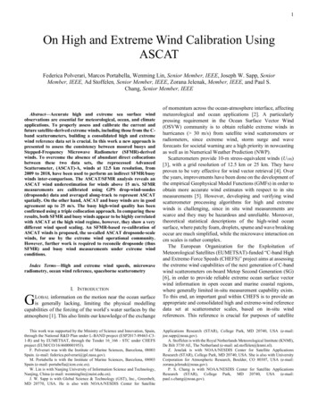
5(a)Fig. 4. (a) Histograms of the different buoy wind speed data sets. The black(blue) curve corresponds to the available MARS (Cwinds) buoy winds whenthe Cwinds (MARS) are missing; the red and magenta curves correspond to thecollocated MARS winds and Cwinds, respectively, when both wind datasources are available. (b) Scatter plot of Cwinds speed versus MARS buoy windspeed. The scores of the correlation coefficient (CC), the bias, and the SD ofthe speed differences are shown in the legend.Karl on September 23rd, 2016 along with the storm BTsecpositions within a few hours from the ASCAT pass (purpleline). The black line in Fig. 3a and Fig. 3b corresponds to theNOAA I2 SFMR flight trajectory in original and storm-motionrelative coordinates, respectively.Note that, the assumption on the “frozen” hurricane structurecannot hold for long time differences. Therefore, the timeseparation t between each SFMR wind acquisition and theASCAT pass, as defined in (1), is taken into account to carryout the wind comparison:) 𝑡 𝑡%)* 𝑡,%&'( (b)(a)(b)(1)where 𝑡,%&'( is the time of the collocated SFMR measurements.We have assessed the 𝑡 impact on the wind comparison bycarrying out an ASCAT/SFMR wind difference analysis atdifferent 𝑡 values, as explained in Section IV. BB. ASCAT/MARS Buoy CollocationTo assess the consistency between MARS and Cwind buoyswinds, we have first carried out a statistical analysis betweenthese two data sets. To this end, five years of Cwinds andMARS buoy winds have been collocated from 2009 to 2014.The wind speed histograms are shown in Fig. 4a for differentcategories, such as: the distribution of the available MARSwind speed when the Cwind data are missing (black line) andvice versa (blue line); the distribution of the collocated Cwinds(purple line) and collocated MARS (red line) winds. Thenumbers of available collocations for each category are 3.4million (black), 2.5 million (red), 2.5 million (magenta) and 4.4million (blue), respectively. As shown by the red and the purplelines, the collocated MARS and Cwinds winds are consistent asthey have very similar distributions, particularly for windsabove 10 m/s. On the other hand, from the difference betweenthe black and the blue curves above 10 m/s, it is clearlydiscernible that the MARS buoy data set has more high windsthan the Cwinds. This is probably due to the fact that the MARSdata set has more buoys at high latitudes (e.g., ODAS). Whenfocusing on the high wind range, as shown in Fig. 4b, Cwindsand MARS buoy data sets are in good agreement, particularlyFig. 5. (a) Scatter-density plot of ASCAT U10S wind speed versus MARS buoyU10N wind speed. The scores of the correlation coefficient (CC), the bias, andthe SD of the speed differences are shown in the legend. (b) Same as shown in(a) but for wind speeds higher than 10 m/s.for winds higher than 15 m/s. Therefore, the MARS buoy windsdata set is favorable for high wind calibration, since it has moredata in the high wind regime and it is seemingly of equal qualityto that of the Cwinds buoy data. For this reason, the MARS dataset is used in this study rather than Cwinds.In order to collocate the MARS buoy winds with the ASCATWVC winds, a temporal distance of 30 minutes along with aspatial distance of 25 km have been used. In case more than oneWVC meets the collocation criteria, the closest WVC to thebuoy acquisition has been used. A total amount of 350,000collocations has been collected. The comparison betweenASCAT and MARS buoys winds has been carried out in thewhole wind speed range as well as by focusing only on the highwind regime. In the latter case, the winds speeds that meet thecondition described in (2) are used:15 ms-. /!"#! 0/%&'(1 25 ms-.(2)where 𝑤*%)* and 𝑤2345 are the ASCAT U10S and the buoyU10N, respectively. A total of 9,700 collocations are collected inthe high wind regime.IV. RESULTSA. ASCAT/Buoy Wind ComparisonThe scatter-density plot of ASCAT wind speed versusMARS buoy wind speed is illustrated in Fig. 5a and Fig. 5b forthe whole wind speed distribution and high winds, respectively.In general, there is very good agreement between ASCAT andMARS wind speeds, with a very high correlation coefficient(CC) of 0.94, a mean bias of -0.12 m/s and a standard deviation(SD) of 1.06 m/s. This is an expected result since buoy windsare used for ASCAT calibration purposes. When focusing onlyon high winds as described in (2), a higher bias of -0.30 m/s( 1.5%) is shown, while the standard deviation is only slightlylarger (1.27 m/s), as compared to the overall distribution. Thisindicates that, on the one hand, there is a good agreement (lowSD) between ASCAT and buoy high winds, and on the otherhand, ASCAT U10S winds slightly underestimate high winds

6(a)(b)(c)Fig. 6. Two-dimensional histograms of ASCAT and collocated SFMR wind speeds averaged over a distance of 12.5 km along track, for 𝑡 1ℎ (a), 𝑡 2ℎ(b), 𝑡 3ℎ (c). The statistical parameters can be found in the legend, such as: correlation coefficient (cc), bias, standard deviation (SD), number of points (Num),root mean square error (rmse).(a)(b)(c)Fig. 7 Same as Fig.6, but for collocated spatially-closest SFMR winds within a maximum radius of 6.25 2 km.Table 1. Triple collocation standard deviation errors for u component (𝜀! ) andthe v component (𝜀" ), at scatterometer scale, assuming that the r2 value is 0.48m-2s-2 for both u and v components.𝜀3 (ms-1)𝜀6 (ms-1)MARSASCATERA51.131.160.570.681.331.37with respect to buoy U10N winds, in line with expectation [3].In order to assess the quality of buoy winds above 15 m/s, wecarried out a triple collocation (hereafter TC) analysis [27],which allows to estimate the errors and the calibrationcoefficients of three sets of collocated measurements. For thisanalysis the buoys (𝑤. ), ASCAT (𝑤1 ), and ERA5 (𝑤7 ) windshave been used. As discussed in [28], to successfully calculatethe individual random errors of each of the three collocated datasets, the representativeness error (𝑟 1 ) needs to be accuratelyestimated. Such error represents the common short-scale truevariance resolved by scatterometer and buoy winds, butunresolved by model winds. Here, the slope approach in [29] isused to estimate the 𝑟 1 value. That is, the 𝑟 1 value that leads towell intercalibrated data sets, such that the regression slopes of𝑤7 versus 𝑤1 , and 𝑤7 versus 𝑤. are both close to one. By usingsuch method, the estimated 𝑟 1 value is 0.48 m-2s-2 for both zonal(u) and meridional (v) wind components. Such value is smallerthan the value presented in [4], which is estimated byintegrating the spectral difference between the scatterometerwind and the ECMWF model winds. In [4], 𝑟 1 is 0.63 m-2s-2 and1.00 m-2s-2 for u and v components, respectively. We haveTable 2. Same as Table 1 but for high wind regime, i.e., using (2). The r2 valueis 0.63 m-2 s-2 and 1.00 m-2s-2 for u and v components respectively.𝜀3 (ms-1)𝜀6 d the impact of varying 𝑟 1 values on the error standarddeviations of the three data sets at the scale resolved by thescatterometer and the results reveal that both 𝜀3 and 𝜀6 are

On the one hand, moored buoy data are generally used as absolute reference to calibrate the scatterometer wind GMFs, however, for very high and extreme winds above 25 m/s, . ASCAT-A collocations and, on the other, buoy and ASCAT-A collocations. Ten NOAA/NESDIS/STAR OSWTyears of reprocessed and stable ASCAT-A surface winds from 2009 to 2018 .