Transcription
This is page 429Printer: Opaque this12Cointegration12.1 IntroductionThe regression theory of Chapter 6 and the VAR models discussed in theprevious chapter are appropriate for modeling I(0) data, like asset returnsor growth rates of macroeconomic time series. Economic theory often implies equilibrium relationships between the levels of time series variablesthat are best described as being I(1). Similarly, arbitrage arguments implythat the I(1) prices of certain financial time series are linked. This chapterintroduces the statistical concept of cointegration that is required to makesense of regression models and VAR models with I(1) data.The chapter is organized as follows. Section 12.2 gives an overview ofthe concepts of spurious regression and cointegration, and introduces theerror correction model as a practical tool for utilizing cointegration withfinancial time series. Section 12.3 discusses residual-based tests for cointegration. Section 12.4 covers regression-based estimation of cointegratingvectors and error correction models. In Section 12.5, the connection between VAR models and cointegration is made, and Johansen’s maximumlikelihood methodology for cointegration modeling is outlined. Some technical details of the Johansen methodology are provided in the appendix tothis chapter.Excellent textbook treatments of the statistical theory of cointegrationare given in Hamilton (1994), Johansen (1995) and Hayashi (2000). Applications of cointegration to finance may be found in Campbell, Lo and
43012. CointegrationMacKinlay (1997), Mills (1999), Alexander (2001), Cochrane (2001) andTsay (2001).12.2 Spurious Regression and Cointegration12.2.1 Spurious RegressionThe time series regression model discussed in Chapter 6 required all variables to be I(0). In this case, the usual statistical results for the linearregression model hold. If some or all of the variables in the regression areI(1) then the usual statistical results may or may not hold1 . One importantcase in which the usual statistical results do not hold is spurious regression when all the regressors are I(1) and not cointegrated. The followingexample illustrates.Example 71 An illustration of spurious regression using simulated dataConsider two independent and not cointegrated I(1) processes y1t andy2t such thatyit yit 1 εit , where εit GW N (0, 1), i 1, 2Following Granger and Newbold (1974), 250 observations for each seriesare simulated and plotted in Figure 12.1 using set.seed(458)e1 rnorm(250)e2 rnorm(250)y1 cumsum(e1)y2 cumsum(e2)tsplot(y1, y2, lty c(1,3))legend(0, 15, c("y1","y2"), lty c(1,3))The data in the graph resemble stock prices or exchange rates. A visualinspection of the data suggests that the levels of the two series are positivelyrelated. Regressing y1t on y2t reinforces this observation: summary(OLS(y1 y2))Call:OLS(formula y1 y2)1 A systematic technical analysis of the linear regression model with I(1) and I(0) variables is given in Sims, Stock and Watson (1990). Hamilton (1994) gives a nice summaryof these results and Stock and Watson (1989) provides useful intuition and examples.
4311512.2 Spurious Regression and Cointegration-15-10-50510y1y2050100150200250FIGURE 12.1. Two simulated independent I(1) processes.Residuals:Min1Q-16.360 tercept)y2Value Std. Error t value Pr( t )6.7445 0.394317.1033 0.00000.4083 0.05088.0352 0.0000Regression Diagnostics:R-Squared 0.2066Adjusted R-Squared 0.2034Durbin-Watson Stat 0.0328Residual standard error: 6.217 on 248 degrees of freedomF-statistic: 64.56 on 1 and 248 degrees of freedom, thep-value is 3.797e-014The estimated slope coefficient is 0.408 with a large t-statistic of 8.035and the regression R2 is moderate at 0.201. The only suspicious statisticis the very low Durbin-Watson statistic suggesting strong residual autocorrelation. These statistics are representative of the spurious regression
43212. Cointegrationphenomenon with I(1) that are not cointegrated. If y1t is regressed on y2t the correct relationship between the two series is revealed summary(OLS(diff(y1) diff(y2)))Call:OLS(formula diff(y1) diff(y2))Residuals:Min1Q Median-3.6632 -0.7706 -0.00743Q0.6983Max2.7184Coefficients:Value Std. Error t value Pr( t )(Intercept) -0.0565 0.0669-0.8447 0.3991diff(y2) 0.0275 0.06420.4290 0.6683Regression Diagnostics:R-Squared 0.0007Adjusted R-Squared -0.0033Durbin-Watson Stat 1.9356Residual standard error: 1.055 on 247 degrees of freedomF-statistic: 0.184 on 1 and 247 degrees of freedom, thep-value is 0.6683Similar results to those above occur if cov(ε1t , ε2t ) 6 0. The levels regression remains spurious (no real long-run common movement in levels),but the differences regression will reflect the non-zero contemporaneouscorrelation between y1t and y2t .Statistical Implications of Spurious RegressionLet Yt (y1t , . . . , ynt )0 denote an (n 1) vector of I(1) time series that are0 0not cointegrated. Using the partition Yt (y1t , Y2t) , consider the leastsquares regression of y1t on Y2t giving the fitted model0y1t β̂2 Y2t ût(12.1)Since y1t is not cointegrated with Y2t (12.1) is a spurious regression andthe true value of β2 is zero. The following results about the behavior of β̂2in the spurious regression (12.1) are due to Phillips (1986): β̂2 does not converge in probability to zero but instead converges indistribution to a non-normal random variable not necessarily centeredat zero. This is the spurious regression phenomenon.
12.2 Spurious Regression and Cointegration433 The usual OLS t-statistics for testing that the elements of β 2 are zerodiverge to as T . Hence, with a large enough sample it willappear that Yt is cointegrated when it is not if the usual asymptoticnormal inference is used. The usual R2 from the regression converges to unity as T sothat the model will appear to fit well even though it is misspecified. Regression with I(1) data only makes sense when the data are cointegrated.12.2.2 CointegrationLet Yt (y1t , . . . , ynt )0 denote an (n 1) vector of I(1) time series. Yt iscointegrated if there exists an (n 1) vector β (β 1 , . . . , β n )0 such thatβ0 Yt β 1 y1t · · · β n ynt I(0)(12.2)In words, the nonstationary time series in Yt are cointegrated if there isa linear combination of them that is stationary or I(0). If some elementsof β are equal to zero then only the subset of the time series in Yt withnon-zero coefficients is cointegrated. The linear combination β0 Yt is oftenmotivated by economic theory and referred to as a long-run equilibriumrelationship. The intuition is that I(1) time series with a long-run equilibrium relationship cannot drift too far apart from the equilibrium becauseeconomic forces will act to restore the equilibrium relationship.NormalizationThe cointegration vector β in (12.2) is not unique since for any scalar cthe linear combination cβ0 Yt β 0 Yt I(0). Hence, some normalizationassumption is required to uniquely identify β. A typical normalization isβ (1, β 2 , . . . , β n )0so that the cointegration relationship may be expressed asβ0 Yt y1t β 2 y2t · · · β n ynt I(0)ory1t β 2 y2t · · · β n ynt ut(12.3)where ut I(0). In (12.3), the error term ut is often referred to as thedisequilibrium error or the cointegrating residual. In long-run equilibrium,the disequilibrium error ut is zero and the long-run equilibrium relationshipisy1t β 2 y2t · · · β n ynt
43412. CointegrationMultiple Cointegrating RelationshipsIf the (n 1) vector Yt is cointegrated there may be 0 r n linearly independent cointegrating vectors. For example, let n 3 and suppose there arer 2 cointegrating vectors β 1 (β 11 , β 12 , β 13 )0 and β2 (β 21 , β 22 , β 23 )0 .Then β01 Yt β 11 y1t β 12 y2t β 13 y3t I(0), β 02 Yt β 21 y1t β 22 y2t β 23 y3t I(0) and the (3 2) matrixµ 0 ¶ µ¶β1β 11 β 12 β 130B β 02β 21 β 22 β 33forms a basis for the space of cointegrating vectors. The linearly independent vectors β 1 and β2 in the cointegrating basis B are not unique unlesssome normalization assumptions are made. Furthermore, any linear combination of β1 and β2 , e.g. β3 c1 β1 c2 β2 where c1 and c2 are constants,is also a cointegrating vector.Examples of Cointegration and Common Trends in Economics andFinanceCointegration naturally arises in economics and finance. In economics, cointegration is most often associated with economic theories that imply equilibrium relationships between time series variables. The permanent incomemodel implies cointegration between consumption and income, with consumption being the common trend. Money demand models imply cointegration between money, income, prices and interest rates. Growth theorymodels imply cointegration between income, consumption and investment,with productivity being the common trend. Purchasing power parity implies cointegration between the nominal exchange rate and foreign anddomestic prices. Covered interest rate parity implies cointegration betweenforward and spot exchange rates. The Fisher equation implies cointegrationbetween nominal interest rates and inflation. The expectations hypothesisof the term structure implies cointegration between nominal interest ratesat different maturities. The equilibrium relationships implied by these economic theories are referred to as long-run equilibrium relationships, becausethe economic forces that act in response to deviations from equilibriiummay take a long time to restore equilibrium. As a result, cointegrationis modeled using long spans of low frequency time series data measuredmonthly, quarterly or annually.In finance, cointegration may be a high frequency relationship or a lowfrequency relationship. Cointegration at a high frequency is motivated byarbitrage arguments. The Law of One Price implies that identical assetsmust sell for the same price to avoid arbitrage opportunities. This impliescointegration between the prices of the same asset trading on differentmarkets, for example. Similar arbitrage arguments imply cointegration between spot and futures prices, and spot and forward prices, and bid and
12.2 Spurious Regression and Cointegration435ask prices. Here the terminology long-run equilibrium relationship is somewhat misleading because the economic forces acting to eliminate arbitrageopportunities work very quickly. Cointegration is appropriately modeledusing short spans of high frequency data in seconds, minutes, hours ordays. Cointegration at a low frequency is motivated by economic equilibrium theories linking assets prices or expected returns to fundamentals. Forexample, the present value model of stock prices states that a stock’s priceis an expected discounted present value of its expected future dividends orearnings. This links the behavior of stock prices at low frequencies to thebehavior of dividends or earnings. In this case, cointegration is modeledusing low frequency data and is used to explain the long-run behavior ofstock prices or expected returns.12.2.3 Cointegration and Common TrendsIf the (n 1) vector time series Yt is cointegrated with 0 r n cointegrating vectors then there are n r common I(1) stochastic trends.To illustrate the duality between cointegration and common trends, letYt (y1t , y2t )0 I(1) and εt (ε1t , ε2t , ε3t )0 I(0) and suppose that Ytis cointegrated with cointegrating vector β (1, β 2 )0 . This cointegrationrelationship may be represented asy1t β2tXε1s ε3ts 1y2t tXε1s ε2ts 1PtThe common stochastic trend is s 1 ε1s . Notice that the cointegratingrelationship annihilates the common stochastic trend:0β Yt β 2tXs 1ε1s ε3t β 2Ã tXs 1ε1s ε2t! ε3t β 2 ε2t I(0).12.2.4 Simulating Cointegrated SystemsCointegrated systems may be conveniently simulated using Phillips’ (1991)triangular representation. For example, consider a bivariate cointegratedsystem for Yt (y1t , y2t )0 with cointegrating vector β (1, β 2 )0 . Atriangular representation has the formy1ty2t β 2 y2t ut , where ut I(0) y2t 1 vt , where vt I(0)(12.4)(12.5)
43612. CointegrationThe first equation describes the long-run equilibrium relationship with anI(0) disequilibrium error ut . The second equation specifies y2t as the common stochastic trend with innovation vt :y2t y20 tXvj .j 1In general, the innovations ut and vt may be contemporaneously and seriallycorrelated. The time series structure of these innovations characterizes theshort-run dynamics of the cointegrated system. The system (12.4)-(12.5)with β 2 1, for example, might be used to model the behavior of thelogarithm of spot and forward prices, spot and futures prices or stock pricesand dividends.Example 72 Simulated bivariate cointegrated systemConsider simulating T 250 observations from the system (12.4)-(12.5)using β (1, 1)0 , ut 0.75ut 1 εt , εt iid N (0, 0.52 ) and vt iid N (0, 0.52 ). The S-PLUS code is set.seed(432)e rmvnorm(250, mean rep(0,2), sd c(0.5,0.5))u.ar1 arima.sim(model list(ar 0.75), innov e[,1])y2 cumsum(e[,2])y1 y2 u.ar1par(mfrow c(2,1))tsplot(y1, y2, lty c(1,3),main "Simulated bivariate cointegrated system",sub "1 cointegrating vector, 1 common trend")legend(0, 7, legend c("y1","y2"), lty c(1,3))tsplot(u.ar1, main "Cointegrating residual")Figure 12.2 shows the simulated data for y1t and y2t along with the cointegrating residual ut y1t y2t . Since y1t and y2t share a common stochastic trend they follow each other closely. The impulse response function forut may be used to determine the speed of adjustment to long-run equilibrium. Since ut is an AR(1) with φ 0.75 the half life of a shock isln(0.5)/ ln(0.75) 2.4 time periods.Next, consider a trivariate cointegrated system for Yt (y1t , y2t , y3t )0 .With a trivariate system there may be one or two cointegrating vectors.With one cointegrating vector there are two common stochastic trends andwith two cointegrating vectors there is one common trend. A triangularrepresentation with one cointegrating vector β (1, β 2 , β 3 )0 and two
12.2 Spurious Regression and Cointegration4378Simulated bivariate cointegrated system-20246y1y20501001502002502002501 cointegrating vector, 1 common trend-1012Cointegrating residual050100150FIGURE 12.2. Simulated bivariate cointegrated system with β (1, 1)0 .stochastic trends isy1ty2ty3t β 2 y2t β 3 y3t ut , where ut I(0) y2t 1 vt , where vt I(0) y3t 1 wt , where wt I(0)(12.6)(12.7)(12.8)The first equation describes the long-run equilibrium and the second andthird equations specify the common stochastic trends. An example of atrivariate cointegrated system with one cointegrating vector is a system ofnominal exchange rates, home country price indices and foreign countryprice indices. A cointegrating vector β (1, 1, 1)0 implies that the realexchange rate is stationary.Example 73 Simulated trivariate cointegrated system with 1 cointegratingvectorThe S-PLUS code for simulating T 250 observation from (12.6)-(12.8)with β (1, 0.5, 0.5)0 , ut 0.75ut 1 εt , εt iid N (0, 0.52 ), vt iid N (0, 0.52 ) and wt iid N (0, 0.52 ) is set.seed(573)e rmvnorm(250, mean rep(0,3), sd c(0.5,0.5,0.5))u1.ar1 arima.sim(model list(ar 0.75), innov e[,1])y2 cumsum(e[,2])
43812. CointegrationSimulated trivariate cointegrated system0510y1y2y30501001502002502002501 cointegrating vector, 2 common trends-1012Cointegrating residual050100150FIGURE 12.3. Simulated trivariate cointegrated system with one cointegratingvector β (1, 0.5, 0.5)0 and two stochastic trends. y3 cumsum(e[,3])y1 0.5*y2 0.5*y3 u1.ar1par(mfrow c(2,1))tsplot(y1, y2, y3, lty c(1,3,4),main "Simulated trivariate cointegrated system",sub "1 cointegrating vector, 2 common trends")legend(0, 12, legend c("y1","y2","y3"), lty c(1,3,4))tsplot(u.ar1, main "Cointegrating residual")Figure 12.3 illustrates the simulated data. Here, y2t and y3t are the twoindependent common trends and y1t 0.5y2t 0.5y3t ut is the averageof the two trends plus an AR(1) residual.Finally, consider a trivariate cointegrated system with two cointegrating vectors and one common stochastic trend. A triangular representation for this system with cointegrating vectors β1 (1, 0, β 13 )0 andβ 2 (0, 1, β 23 )0 isy1ty2ty3t β 13 y3t ut , where ut I(0) β 23 y3t vt , where vt I(0) y3t 1 wt , where wt I(0)(12.9)(12.10)(12.11)Here the first two equations describe two long-run equilibrium relationsand the third equation gives the common stochastic trend. An example in
12.2 Spurious Regression and Cointegration439finance of such a system is the term structure of interest rates where y3represents the short rate and y1 and y2 represent two different long rates.The cointegrating relationships would indicate that the spreads betweenthe long and short rates are stationary.Example 74 Simulated trivariate cointegrated system with 2 cointegratingvectorsThe S-PLUS code for simulating T 250 observation from (12.9)-(12.11)with β1 (1, 0, 1)0 , β 2 (0, 1, 1)0 , ut 0.75ut 1 εt , εt iid N (0, 0.52 ),vt 0.75vt 1 ηt , η t iid N (0, 0.52 ) and wt iid N (0, 0.52 ) is set.seed(573)e rmvnorm(250,mean rep(0,3), sd c(0.5,0.5,0.5))u.ar1 arima.sim(model list(ar 0.75), innov e[,1])v.ar1 arima.sim(model list(ar 0.75), innov e[,2])y3 cumsum(e[,3])y1 y3 u.ar1y2 y3 v.ar1par(mfrow c(2,1))tsplot(y1, y2, y3, lty c(1,3,4),main "Simulated trivariate cointegrated system",sub "2 cointegrating vectors, 1 common trend")legend(0, 10, legend c("y1","y2","y3"), lty c(1,3,4))tsplot(u.ar1, v.ar1, lty c(1,3),main "Cointegrated residuals")legend(0, -1, legend c("u","v"), lty c(1,3))12.2.5 Cointegration and Error Correction ModelsConsider a bivariate I(1) vector Yt (y1t , y2t )0 and assume that Yt iscointegrated with cointegrating vector β (1, β 2 )0 so that β 0 Yt y1t β 2 y2t is I(0). In an extremely influential and important paper, Engle andGranger (1987) showed that cointegration implies the existence of an errorcorrection model (ECM) of the form y1t c1 α1 (y1t 1 β 2 y2t 1 )X jX j ψ 11 y1t j ψ 12 y2t j ε1tj y2tj c2 α2 (y1t 1 β 2 y2t 1 )X jX ψ 21 y1t j ψ 222 y2t j ε2tj(12.12)(12.13)jthat describes the dynamic behavior of y1t and y2t . The ECM links thelong-run equilibrium relationship implied by cointegration with the shortrun dynamic adjustment mechanism that describes how the variables react
44012. Cointegration10Simulated trivariate cointegrated system05y1y2y30501001502002502002502 cointegrating vectors, 1 common trend-101Cointegrated residuals-2uv050100150FIGURE 12.4. Simulated trivatiate cointegrated system with two cointegratingvectors β 1 (1, 0, 1)0 , β 2 (0, 1, 1)0 and one common trend.when they move out of long-run equilibrium. This ECM makes the conceptof cointegration useful for modeling financial time series.Example 75 Bivariate ECM for stock prices and dividendsAs an example of an ECM, let st denote the log of stock prices and dtdenote the log of dividends and assume that Yt (st , dt )0 is I(1). If thelog dividend-price ratio is I(0) then the logs of stock prices and dividendsare cointegrated with β (1, 1)0 . That is, the long-run equilibrium isdt st µ utwhere µ is the mean of the log dividend-price ratio, and ut is an I(0) randomvariable representing the dynamic behavior of the log dividend-price ratio(disequilibrium error). Suppose the ECM has the form st dt cs αs (dt 1 st 1 µ) εst cd αd (dt 1 st 1 µ) εdtwhere cs 0 and cd 0. The first equation relates the growth rate ofdividends to the lagged disequilibrium error dt 1 st 1 µ, and the secondequation relates the growth rate of stock prices to the lagged disequilibriumas well. The reactions of st and dt to the disequilibrium error are capturedby the adjustment coefficients αs and αd .
12.2 Spurious Regression and Cointegration441Consider the special case of (12.12)-(12.13) where αd 0 and αs 0.5.The ECM equations become st dt cs 0.5(dt 1 st 1 µ) εst , cd εdt .so that only st responds to the lagged disequilibrium error. Notice thatE[ st Yt 1 ] cs 0.5(dt 1 st 1 µ) and E[ dt Yt 1 ] cd . Considerthree situations:1. dt 1 st 1 µ 0. Then E[ st Yt 1 ] cs and E[ dt Yt 1 ] cd , sothat cs and cd represent the growth rates of stock prices and dividendsin long-run equilibrium.2. dt 1 st 1 µ 0. Then E[ st Yt 1 ] cs 0.5(dt 1 st 1 µ) cs . Here the dividend yield has increased above its long-run mean(positive disequilibrium error) and the ECM predicts that st will growfaster than its long-run rate to restore the dividend yield to its longrun mean. Notice that the magnitude of the adjustment coefficientαs 0.5 controls the speed at which st responds to the disequilibriumerror.3. dt 1 st 1 µ 0. Then E[ st Yt 1 ] cs 0.5(dt 1 st 1 µ) cs . Here the dividend yield has decreased below its long-run mean(negative disequilibrium error) and the ECM predicts that st willgrow more slowly than its long-run rate to restore the dividend yieldto its long-run mean.In Case 1, there is no expected adjustment since the model was in longrun equilibrium in the previous period. In Case 2, the model was abovelong-run equilibrium last period so the expected adjustment in st is downward toward equilibrium. In Case 3, the model was below long-run equilibrium last period and so the expected adjustment is upward toward theequilibrium. This discussion illustrates why the model is called an error correction model. When the variables are out of long-run equilibrium, thereare economic forces, captured by the adjustment coefficients, that pushthe model back to long-run equilibrium. The speed of adjustment towardequilibrium is determined by the magnitude of αs . In the present example,αs 0.5 which implies that roughly one half of the disequilibrium erroris corrected in one time period. If αs 1 then the entire disequilibriumis corrected in one period. If αs 1.5 then the correction overshoots thelong-run equilibrium.
44212. Cointegration12.3 Residual-Based Tests for CointegrationLet the (n 1) vector Yt be I(1). Recall, Yt is cointegrated with 0 r ncointegrating vectors if there exists an (r n) matrix B0 such that 0u1tβ1 Yt . .B0 Yt . I(0).β0r YturtTesting for cointegration may be thought of as testing for the existenceof long-run equilibria among the elements of Yt . Cointegration tests covertwo situations: There is at most one cointegrating vector There are possibly 0 r n cointegrating vectors.The first case was originally considered by Engle and Granger (1986) andthey developed a simple two-step residual-based testing procedure basedon regression techniques. The second case was originally considered by Johansen (1988) who developed a sophisticated sequential procedure for determining the existence of cointegration and for determining the number ofcointegrating relationships based on maximum likelihood techniques. Thissection explains Engle and Granger’s two-step procedure. Johansen’s moregeneral procedure will be discussed later on.Engle and Granger’s two-step procedure for determining if the (n 1)vector β is a cointegrating vector is as follows: Form the cointegrating residual β0 Yt ut Perform a unit root test on ut to determine if it is I(0).The null hypothesis in the Engle-Granger procedure is no-cointegration andthe alternative is cointegration. There are two cases to consider. In the firstcase, the proposed cointegrating vector β is pre-specified (not estimated).For example, economic theory may imply specific values for the elementsin β such as β (1, 1)0 . The cointegrating residual is then readily constructed using the prespecified cointegrating vector. In the second case, theproposed cointegrating vector is estimated from the data and an estimate0of the cointegrating residual β̂ Yt ût is formed. Tests for cointegrationusing a pre-specified cointegrating vector are generally much more powerfulthan tests employing an estimated vector.12.3.1 Testing for Cointegration When the CointegratingVector Is Pre-specifiedLet Yt denote an (n 1) vector of I(1) time series, let β denote an (n 1)prespecified cointegrating vector and let ut β0 Yt denote the prespecified
12.3 Residual-Based Tests for Cointegration4430.00Log US/CA exchange rate data-0.35-0.15spotforward1976 1977 1978 1979 1980 1981 1982 1983 1984 1985 1986 1987 1988 1989 1990 1991 1992 1993 1994 1995 1996-0.0040.0000.004US/CA 30-day interest rate differential1976 1977 1978 1979 1980 1981 1982 1983 1984 1985 1986 1987 1988 1989 1990 1991 1992 1993 1994 1995 1996FIGURE 12.5. Log of US/CA spot and 30-day exchange rates and 30-day interestrate differential.cointegrating residual. The hypotheses to be tested areH0H1: ut β0 Yt I(1) (no cointegration): ut β0 Yt I(0) (cointegration)(12.14)Any unit root test statistic may be used to evaluate the above hypotheses.The most popular choices are the ADF and PP statistics. Cointegration isfound if the unit root test rejects the no-cointegration null. It should be keptin mind, however, that the cointegrating residual may include deterministicterms (constant or trend) and the unit root tests should account for theseterms accordingly. See Chapter 4 for details about the application of unitroot tests.Example 76 Testing for cointegration between spot and forward exchangerates using a known cointegrating vectorIn international finance, the covered interest rate parity arbitrage relationship states that the difference between the logarithm of spot andforward exchange rates is equal to the difference between nominal domestic and foreign interest rates. It seems reasonable to believe that interestrate spreads are I(0) which implies that spot and forward rates are cointegrated with cointegrating vector β (1, 1)0 . To illustrate, consider thelog monthly spot, st , and 30 day forward, ft , exchange rates between the
44412. CointegrationUS and Canada over the period February 1976 through June 1996 takenfrom the S FinMetrics “timeSeries” object lexrates.dat uscn.s lexrates.dat[,"USCNS"]uscn.s@title "Log of US/CA spot exchange rate"uscn.f lexrates.dat[,"USCNF"]uscn.f@title "Log of US/CA 30-day forward exchange rate"u uscn.s - uscn.fcolIds(u) "USCNID"u@title "US/CA 30-day interest rate differential"The interest rate differential is constructed using the pre-specified cointegrating vector β (1, 1)0 as ut st ft . The spot and forward exchangerates and interest rate differential are illustrated in Figure 12.5. Visually,the spot and forward exchange rates clearly share a common trend and theinterest rate differential appears to be I(0). In addition, there is no clear deterministic trend behavior in the exchange rates. The S FinMetrics function unitroot may be used to test the null hypothesis that st and ft arenot cointegrated (ut I(1)). The ADF t-test based on 11 lags and a constant in the test regression leads to the rejection at the 5% level of thehypothesis that st and ft are not cointegrated with cointegrating vectorβ (1, 1)0 : unitroot(u, trend "c", method "adf", lags 11)Test for Unit Root: Augmented DF TestNull Hypothesis:Type of Test:Test Statistic:P-value:there is a unit g4lag5lag6-0.1464 -0.1171 -0.0702 -0.1008 -0.1234 -0.1940lag8-0.1235lag90.0550lag10lag11 constant0.2106 -0.1382 0.0002Degrees of freedom: 234 total; 222 residualTime period: from Jan 1977 to Jun 1996Residual standard error: 8.595e-4lag70.0128
12.3 Residual-Based Tests for Cointegration44512.3.2 Testing for Cointegration When the CointegratingVector Is EstimatedLet Yt denote an (n 1) vector of I(1) time series and let β denote an(n 1) unknown cointegrating vector. The hypotheses to be tested aregiven in (12.14). Since β is unknown, to use the Engle-Granger procedureit must be first estimated from the data. Before β can be estimated somenormalization assumption must be made to uniquely identify it. A commonnormalization is to specify the first element in Yt as the dependent variable0 0and the rest as the explanatory variables. Then Yt (y1t , Y2t) where0Y2t (y2t , . . . , ynt ) is an ((n 1) 1) vector and the cointegrating vectoris normalized as β (1, β02 )0 . Engle and Granger propose estimating thenormalized cointegrating vector β2 by least squares from the regressiony1t c β02 Y2t ut(12.15)and testing the no-cointegration hypothesis (12.14) with a unit root testusing the estimated cointegrating residualût y1t ĉ β̂ 2 Y2t(12.16)where ĉ and β̂2 are the least squares estimates of c and β2 . The unit roottest regression in this case is without deterministic terms (constant or constant and trend). Phillips and Ouliaris (1990) show that ADF and PP unitroot tests (t-tests and normalized bias) applied to the estimated cointegrating residual (12.16) do not have the usual Dickey-Fuller distributions underthe null hypothesis (12.14) of no-cointegration. Instead, due to the spuriousregression phenomenon under the null hypothesis (12.14), the distributionof the ADF and PP unit root tests have asymptotic distributions that arefunctions of Wiener processes that depend on the deterministic terms inthe regression (12.15) used to estimate β2 and the number of variables,n 1, in Y2t . These distributions are known as the Phillips-Ouliaris (PO)distributions, and are described in Phillips and Ouliaris (1990). To furthercomplicate matters, Hansen (1992) showed the appropriate PO distributions of the ADF and PP unit root tests applied to the residuals (12.16)also depend on the trend behavior of y1t and Y2t as follows:Case I: Y2t and y1t are both I(1) without drift. The ADF and PP unitroot test statistics follow the PO distributions, adjusted for a constant, with dimension parameter n 1.Case II: Y2t is I
The regression theory of Chapter 6 and the VAR models discussed in the previous chapter are appropriate for modeling I(0) data, like asset returns or growth rates of macroeconomic time series. Economic theory often im-plies equilibrium relationships between the levels of time series variables that are best described as being I(1).