WIXLIB

5BOX 1: Mathematical definitionsEntropy. The entropy of a random variable r with a probability density p(r) is a measure of our uncertainty about the variableZand is defined as:H(r) p(r) · log p(r) dr(1)The conditional entropy of a random variable r given another random variable θ is defined as:ZH(r θ) p(r, θ) · log p(r θ) dr dθ(2)Mutual information. The mutual information (MI) I(r; θ) between response r and stimulus θ measures the information thatthe response conveys about the stimulus (and vice versa). The MI can be thought of as the shared entropy, or entropyoverlap, that is the number of bits by which the entropy H(r, θ) of the joint distribution of both variables is smaller than thesum of their individual entropies H(r) and H(θ):I(r; θ) H(r) H(θ) H(r, θ)(3)Equivalently, the MI is the reduction of the entropy of one of the variables when we learn about the other:I(r; θ) H(r) H(r θ) H(θ) H(θ r)Note that MI depends on the distribution of both variables. In more explicit terms, the MI can be expressed as:Z Zp(r, θ)I(r; θ) p(r, θ) logdrdθ.p(r)p(θ)(4)(5)Fisher information. The Fisher information (FI) of a neural population code is a function of the stimulus. For each location instimulus space, the FI reflects how sensitive the code is to local changes of the stimulus. Assume a population of N neuronsencoding stimulus variable θ, with tuning curves fi . The population response is denoted as r. The FI can be defined asZd2J(θ) 2 log p(r θ)p(r)dr.(6)dθIf θ is a vector, rather than a scalar, description of the stimulus, J(θ) becomes the FI matrix, characterizing the magnitudeof the response pattern change for all directions in stimulus space. The FI of a neuron is determined by the neuron’s tuningcurve and noise characteristics. Assuming Poisson spiking, and tuning curve f (θ), where θ is the encoded stimulus property,the Fisher information J(θ) can be computed asJ(θ) f 0 (θ)2.f (θ)(7)Under the assumption of additive stimulus-independent Gaussian noise (with noise variance equal to 1), the Fisher information is simply the squared slope of the tuning curveJ(θ) f 0 (θ)2 .(8)For a neural population, if neurons have independent noise, the population FI is simply the sum of the FI for individualneurons. With correlated noise, evaluating the FI is more complicated as it depends on the correlation structure. FI dependson the specific parameterization of the stimulus space. More precisely, when θ is reparameterized as θ̃, the following relationqpJ(θ)dθ J(θ̃)dθ̃.(9)holds:Discrimination threshold. The square root of the Fisher information provides a lower bound on the discrimination thresholdδ(θ) in fine discrimination taskspδ(θ) C/ J(θ),(10)where C is a constant dependent on the definition of the psychophysical discrimination threshold.Variance-stabilizing transformation. For independent Poisson noise, we can apply a square-root transformation to anindividual neuron’s response ri [139, 140]. The resulting response will have approximately constant variance independentof firing rate. In general, assuming the variance of ri is a smooth function g(·) of its mean µ , one could first stabilize thevariance by applying the following transformation to obtain r i and the statements below would apply to r i .Z ri1pr i dµg(µ)(11)

622.1A dual perspectiveTuning determines mutual information and Fisher informationA tuning curve tells us how the mean activity level of an individual neuron varies depending on a stimulusproperty. The tuning curve, thus, defines how the stimulus property is encoded in the neuron’s activity.Conversely, knowing the activity of the neuron may enable us to decode the stimulus property. Howinformative the neural response is depends on the shape of the tuning curve. A flat tuning curve, oftendescribed as a lack of tuning, would render the response uninformative. If the neuron is tuned, it contains some information about the stimulus property. However, a single neuron may respond similarly todifferent stimuli. For example, a neuron tuned to stimulus orientation may respond equally to two stimulidiffering from its preferred orientation in either direction by the same angle. The resulting ambiguity maybe resolved by decoding from multiple neurons.For a population of neurons, the tuning function f (θ) can be defined as the expected value of the response pattern r given stimulus parameter θ:f (θ) Er p(r θ) [r] E[r θ].(12)In the special case of additive noise with mean zero, the response pattern obtains as r f (θ) , wheref (θ) is the encoding model that defines the tuning function for each neuron and is the noise.We can quantify the information contained in the neural code about the stimulus using the mutual information or the Fisher information, two measures that have been widely used in computational neuroscience. Mutual information (MI) is a key quantity of information theory that measures how muchinformation one random variable contains about another random variable [86]. The MI I(r; θ) measuresthe information the response r conveys about the stimulus θ (Box 1). Computing the MI requires assuming a prior p(θ) over the stimuli, because the MI is a function of the joint distribution p(r, θ) p(r θ) · p(θ)of stimulus and response.Over the past few decades, MI has been used extensively in neuroscience [87, 88, 89, 90]. For example,studies have aimed to quantify the amount of information conveyed by neurons about sensory stimuli[91, 87, 90, 89, 92, 93]. MI has also been used as an objective function to be maximized, so as toderive an efficient encoding of a stimulus property in a limited number of neurons ([94, 95, 96, 97, 98]).If a neural code optimizes the MI, the code must reflect the statistical structure of the environment. Forexample, in an MI-maximizing code, frequent stimuli should be encoded with greater precision. Oncea prior over the stimuli, a functional form of the encoding, and a noise model have been specified, thejoint distribution of stimulus and response is defined, and the MI can be computed. The parameters ofthe encoding can then be optimized to maximize MI [99, 100, 101]. If the tuning functions that maximizeMI match those observed in brains, the function to convey information about the stimulus may explainwhy the neurons exhibit their particular tuning [101, 102, 103, 104, 105, 106, 107, 90, 108, 109]. Theapplications of information theory in neuroscience have been the subject of previous reviews ([88, 89,

7110]).The MI provides a measure of the overall information the response conveys about the stimulus. It canbe thought of as the expected value of the reduction of the uncertainty about the stimulus that an idealobserver experiences when given the response, where the expectation is across the distribution of stimuli. However, the MI does not capture how the fidelity of the encoding depends on the stimulus. Someauthors have proposed stimulus-specific variants of MI [111, 112, 16, 113].Another stimulus-specific measure of information in the neural response is the Fisher information (FI).The FI has deep roots in statistical estimation theory [85, 114] and plays a central role in the frameworkwe propose here. The FI captures the precision with which a stimulus property is encoded in the vicinityof a particular value of the property [115, 116, 117, 95, 109]. An efficient code for a particular stimulusdistribution will dedicate more resources to frequent stimuli and encode these with greater precision. TheFI is a function of the stimulus and reflects the variation of the precision of the encoding across differentvalues of the stimulus property.A large body of work has studied how tuning parameters, such as tuning width and firing rate, are relatedto the FI [118, 119, 115, 120, 121, 122, 123, 124]. The FI is proportional to the squared slope of the tuningcurve when the noise is Gaussian and additive (Box 1). When the noise follows a Poisson distribution, theFI is the squared slope of the tuning curve divided by the firing rate. Beyond single neurons and particularnoise distributions, the FI provides a general stimulus-specific measure that characterizes coding fidelityof a neuronal population under various noise distributions. The FI sums across neurons, to yield theneural-population FI, if the neurons have independent noise. However, when the noise is correlatedbetween neurons, the Fisher information is more difficult to compute [125, 126, 127, 128, 129, 130]. Thisis still an active area of research [131, 132, 133, 134, 135, 121, 136, 261], and some progress has beenreviewed in [137, 138].2.2Tuning determines geometryA tuning curve describes the encoding of a stimulus property in an individual neuron. When we considera population of neurons, we can think of the response pattern across the n neurons as a point in an ndimensional space. Let’s assume the tuning curves are continuous functions of the stimulus property. Aswe sweep through the values of the stimulus property, the response pattern moves along a 1-dimensionalmanifold in the neural response space. Now imagine that stimuli vary along d property dimensions thatare all encoded in the neural responses with continuous tuning curves. As we move in the d-dimensionalstimulus-property space, the response pattern moves along a d-dimensional neural response manifold(Box 2).

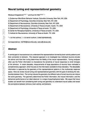
8BOX 2: Neural response manifoldA neural response manifold is a set of response patterns elicited by a range of stimuli [141, 142, 54, 143]. In neuroscience,we often think of a curved hypersurface of the neural response space within which each stimulus has its unique location.The mathematical notion of manifold implies that the set of neural response patterns is locally homeomorphic to a Euclideanspace. This notion is particularly helpful when (1) the tuning curves are continuous, (2) the mapping between d-vectors ofstimulus properties and n-vectors of neural responses is bijective, and (3) we neglect the noise. Under these conditions, theset of neural response patterns is homeomorphic to the particular Euclidean space spanned by the stimulus properties, andwe can imagine mapping the stimulus space onto a hypersurface (which might be nonlinear, but will not intersect itself) in themultivariate response space.Consider a pair of neurons encoding orientation with sinusoidal tuning curves. Because both tuning curves are continuous,the response will vary continuously and cyclicly as the stimulus rotates. When the phases of the tuning curves are offset by90 , the response manifold is a perfect circle (a). As the phase offset increases, the manifold gradually morphs into an ellipsewith increasing aspect ratio (b, c). The shape of the manifold depends on the exact shape of the tuning curves. Panel (d)shows a crescent-like response manifold, induced by two von Mises tuning curves. For certain tuning functions, the responsehypersurface may self-intersect (e). In the neighborhood of the self-intersection, the hypersurface is not homeomorphic toany Euclidean space, and thus not a manifold. However, adding one additional neuron (neuron 3 in f), disentangles thehypersurface, and renders it a manifold again. The width of bell-shaped tuning curves (g and h) substantially modulatesthe geometry of the manifold, with narrower tuning curves (h) leading to a manifold that is highly curved and requires ahigher-dimensional linear subspace to explain most the variance (Fig. 1, compare rows a and b, rightmost column).These examples neglect the presence of noise. When the responses are noisy, they may still form a manifold, but not ad-dimensional manifold, whose dimensions correspond to the d stimulus properties of interest. Despite these caveats, thenotion of manifold appears useful, because it enables us to see the response patterns elicited by a d-dimensional space ofstimuli as a d-dimensional sheet in the multivariate response space [141, 142, 53, 54, 143, 144, 84, 145].1neuron 2000neuron 11-20c1102-202210neuron 1100neuron 1 1d1210-20e10211000neuron 111f2-2011022-2g30210.50neuron 1101311ne 0.50.5ur1on 0 0ron2neu0-220h131021neuron 311neuron 30stimulus2neuron 31neuron 2bneuron 2neuron 1neuron 20neuron 2neuron 21firing ratea-2201210.50.51neu 0.5ron20.51rneuon 1011ne 0.50.51uron 2 0 0 neuronThe concept of a neural response manifold [141, 142] helps us relate a uni-dimensional or multidimensional stimulus space to a high-dimensional neural response space. To understand the code, we mustunderstand the geometry of the neural response manifold. As we saw above, the FI tells us the magnitude of the response pattern change associated with a local move in stimulus space around any givenlocation θ. To define the representational geometry, however, we need a global characterization. Weneed to know the magnitudes of the response pattern changes associated with arbitrary moves from anystimulus to any other stimulus. The geometry is determined by the distances in multivariate responsespace that separate the representations of any two stimuli. The tuning curves define the response patterns, from which we can compute the representational distances.We could simply use the Euclidean distances d(θi , θj ) for all pairs (i, j) of stimuli, which can be computedon the basis of the tuning functions alone to define the representational geometry:d(θi , θj ) kf (θi ) f (θj )k.(13)

9However, we would like to define the representational geometry in a way that reflects the discriminability of the stimuli. The discriminability could be defined in various ways, for example as the accuracyof a Bayes-optimal decoder, as the accuracy or d0 of a linear decoder, or as the mutual informationbetween stimulus and neural response. The Euclidean distance between stimulus representations ismonotonically related to all these measures of the discriminability when the noise distribution is isotropic,Gaussian, and stimulus-independent. When the noise is anisotropic (and still Gaussian and stimulusindependent), we can replace the Euclidean distance with the Mahalanobis distanceq1dM ahal (θi , θj ) [f (θi ) f (θj )]T Σ 1 [f (θi ) f (θj )] kΣ 2 [f (θi ) f (θj )]k,(14)where Σ is the noise covariance matrix. The Mahalanobis distance will be monotonically related to thediscriminability [75].When the noise is Poisson and independent between neurons, a square-root transform can be usedto stabilize the variance and render the joint noise density approximately Gaussian and isotropic (Box1, [146]). How to best deal with non-Gaussian (e.g. Poisson) stimulus-dependent noise is an unresolvedissue.We have seen that the geometry of the representation depends on the tuning and the noise and can becharacterized by a representational distance matrix. Changing the tuning will usually change the representational geometry. Consider the encoding of stimulus orientation by a population of neurons thathave von Mises tuning with constant width of the tuning curves and a uniform distribution of preferredorientations. Since orientations form a cyclic set and the tuning curves are continuous, the set of representational patterns must form a cycle (Fig. 1a). However, two uniform neural population codes withdifferent tuning widths will have distinct representational geometries.With narrow tuning width (Fig. 1a), a given stimulus drives a sparse set of neurons. For intuition onthis narrow tuning regime, imagine a labeled-line code, where each neuron responds to a particularstimulus from a finite set (one neuron for each stimulus). As we move through the stimulus set, wedrive each neuron in turn. The set of response patterns, thus, is embedded in a linear subspace of thesame dimensionality as the number of neurons. Note also that narrow tuning yields a “splitter" code,i.e., a code that is equally sensitive to small and large orientation changes. Orientations differing by 30degrees (π/6 radians) might elicit non-overlapping response patterns and would, thus, be as distant inthe representational space as orientations differing by 90 degrees (π/2 radians, Fig. 1a, second-to-lastcolumn).With wide tuning width (Fig. 1b), the geometry approximates a circle. It would be exactly a circlefor two neurons with sinusoidal tuning with a π/4 shift in preferred orientation (where π is the cycleperiod for stimulus orientation), and in the limit of an infinite number of neurons with sinusoidal tuning(with preferred orientations drawn from a uniform distribution). For von Mises tuning curves and finitenumbers of neurons, wide tuning entails a geometry approximating a circle, with most of the varianceof the set of response patterns explained by the first two principal components. Wide tuning yields a“lumper" code, i.e., a code that is more sensitive to global orientation changes, than to local changes.

10Orientations differing by 30 degrees will elicit overlapping response patterns and would be much closerin the representational space than orientations differing by 90 degrees (Fig. 1b, right column).If we make the gain or the width of the tuning curves non-uniform across orientations, the geometry isdistorted with stimuli spreading out in representational space in regions of high Fisher information andhuddling together in regions of low Fisher information (as illustrated in the RDM and MDS in Fig. 1c).This section explained how a set of tuning functions induces a representational geometry. We definedthe geometry by its sufficient statistic, the representational distance matrix. The distances are measuredafter a transformation that renders the noise isotropic. We will see below that the distance matrix thencaptures all information contained in the code. Importantly, it also captures important aspects of theformat in which the information is encoded. For example, knowing the geometry and the noise distributionenables us to predict what information can be read out from the code with a linear decoder (or in fact anygiven nonlinear decoder capable of a linear transform).2.3Geometry does not determine tuningWe have seen that the set of tuning curves determines the geometry (given the noise distribution). Theconverse does not hold: The geometry does not determine the set of tuning curves. To understand this,let us assume that the noise is isotropic (or has been rendered isotropic by a whitening transform). It iseasy to see that rotating the ensemble of points corresponding to the representational patterns will leavethe geometry unchanged. Such a rotation could simply exchange tuning curves between neurons, whileleaving the set of tuning curves the same. In general, however, a rotation of the ensemble of points willsubstantially and qualitatively change the set of tuning curves (Fig. 1, compare b and d). The ne

to be represented by the brain. Like a radio tuned to a particular frequency to select a station, a "tuned" neuron [3] may selectively respond to stimuli within a particular band of some stimulus variable, which could be a spatial or temporal frequency, or some other property of the stimulus