Transcription
MolecularDriving ForcesMolecularDriving ForcesStatistical Thermodynamics in Biology,Chemistry, Physics, and NanoscienceSecond .comISBN 978-0-8153-4430-89 780815 344308Ken A. DillSarina Bromberg
Garland ScienceVice President: Denise SchanckSenior Editor: Michael MoralesAssistant Editor: Monica ToledoProduction Editor: H.M. (Mac) ClarkeIllustrator & Cover Design: Xavier StudioCopyeditor: H.M. (Mac) ClarkeTypesetting: Techset Composition LimitedProofreader: Sally HuishIndexer: Merrall-Ross International, Ltd.Ken A. Dill is Professor and Director of the Laufer Center for Physical and QuantitativeBiology at Stony Brook University. He received his undergraduate training at MIT, his PhDfrom the University of California, San Diego, did postdoctoral work at Stanford, and wasProfessor at the University of California, San Francisco until 2010. A researcher instatistical mechanics and protein folding, he has been the President of the BiophysicalSociety and is a member of the US National Academy of Sciences.Sarina Bromberg received her BFA at the Cooper Union for the Advancement of Scienceand Art, her PhD in molecular biophysics from Wesleyan University, and her postdoctoraltraining at the University of California, San Francisco. She writes, edits, and illustratesscientific textbooks.Dirk Stigter (1924–2010) received his PhD from the State University of Utrecht, TheNetherlands, and did postdoctoral work at the University of Oregon, Eugene. 2011 by Garland Science, Taylor & Francis Group, LLCThis book contains information obtained from authentic and highly regarded sources.Reprinted material is quoted with permission, and sources are indicated. A wide variety ofreferences are listed. Reasonable efforts have been made to publish reliable data andinformation, but the author and the publisher cannot assume responsibility for thevalidity of all materials or for the consequences of their use. All rights reserved. No part ofthis publication may be reproduced, stored in a retrieval system, or transmitted in anyform or by any means—graphic, electronic, or mechanical, including photocopying,recording, taping, or information storage and retrieval systems—without permission of thecopyright holder.ISBN 978-0-8153-4430-8Library of Congress Cataloging-in-Publication DataDill, Ken A.Molecular driving forces : statistical thermodynamics in chemistry,physics, biology, and nanoscience / Ken Dill, Sarina Bromberg. – – 2nd ed.p. cm.Includes index.ISBN 978-0-8153-4430-8 (pbk.)1. Statistical thermodynamics. I. Bromberg, Sarina. II. Title.QC311.5.D55 2010536’.7– –dc222010034322Published by Garland Science, Taylor & Francis Group, LLC, an informa business,270 Madison Avenue, New York, NY 10016, USA, and2 Park Square, Milton Park, Abingdon, OX14 4RN, UKPrinted in the United States of America15 14 13 12 11 10 9 8 7 6 5 4 3 2 1Visit our web site at http://www.garlandscience.com
1Principles ofProbabilityThe Principles of Probability Arethe Foundations of EntropyFluids flow, boil, freeze, and evaporate. Solids melt and deform. Oil and waterdon’t mix. Metals and semiconductors conduct electricity. Crystals grow.Chemicals react and rearrange, take up heat, and give it off. Rubber stretchesand retracts. Proteins catalyze biological reactions. What forces drive these processes? This question is addressed by statistical thermodynamics, a set of toolsfor modeling molecular forces and behavior, and a language for interpretingexperiments.The challenge in understanding these behaviors is that the properties thatcan be measured and controlled, such as density, temperature, pressure, heatcapacity, molecular radius, or equilibrium constants, do not predict the tendencies and equilibria of systems in a simple and direct way. To predict equilibria,we must step into a different world, where we use the language of energy,entropy, enthalpy, and free energy. Measuring the density of liquid water justbelow its boiling temperature does not hint at the surprise that, just a fewdegrees higher, above the boiling temperature, the density suddenly dropsmore than a thousandfold. To predict density changes and other measurableproperties, you need to know about the driving forces, the entropies and energies. We begin with entropy.Entropy is one of the most fundamental concepts in statistical thermodynamics. It describes the tendency of matter toward disorder. Entropy explains1
how expanding gases drive car engines, liquids mix, rubber bands retract, heatflows from hot objects to cold objects, and protein molecules tangle togetherin some disease states. The concepts that we introduce in this chapter, probability, multiplicity, combinatorics, averages, and distribution functions, providea foundation for describing entropy.What Is Probability?Here are two statements of probability. In 1990, the probability that a person inthe United States was a scientist or an engineer was 1/250. That is, there wereabout a million scientists and engineers out of a total of about 250 millionpeople. In 1992, the probability that a child under 13 years old in the UnitedStates ate a fast-food hamburger on any given day was 1/30 [1].Let’s generalize. Suppose that the possible outcomes fall into categories A,B, or C. ‘Event’ and ‘outcome’ are generic terms. An event might be the flippingof a coin, resulting in heads or tails. Alternatively, it might be one of the possibleconformations of a molecule. Suppose that outcome A occurs 20% of the time,B 50% of the time, and C 30% of the time. Then the probability of A is 0.20, theprobability of B is 0.50, and the probability of C is 0.30.The definition of probability is as follows: If N is the total number of possible outcomes, and nA of the outcomes fall into category A, then pA , the probability of outcome A, is!"nA.(1.1)pA NProbabilities are quantities in the range from zero to one. If only one outcomeis possible, the process is deterministic—the outcome has a probability of one.An outcome that never occurs has a probability of zero.Probabilities can be computed for different combinations of events. Consider one roll of a six-sided die, for example (die, unfortunately, is the singularof dice). The probability that a 4 appears face up is 1/6 because there are N 6possible outcomes and only n4 1 of them is a 4. But suppose you roll a sixsided die three times. You may ask for the probability that you will observe thesequence of two 3’s followed by one 4. Or you may ask for the probability ofrolling two 2’s and one 6 in any order. The rules of probability and combinatorics provide the machinery for calculating such probabilities. Here we definethe relationships among events that we need to formulate these rules.Definitions: Relationships Among EventsMutually Exclusive. Outcomes A1 , A2 , . . . , At are mutually exclusive if theoccurrence of each one of them precludes the occurrence of all the others. If Aand B are mutually exclusive, then if A occurs, B does not. If B occurs, A doesnot. For example, on a single die roll, 1 and 3 are mutually exclusive becauseonly one number can appear face up each time the die is rolled.Collectively Exhaustive. Outcomes A1 , A2 , . . . , At are collectively exhaustive if they constitute the entire set of possibilities, and no other outcomes arepossible. For example, [heads, tails] is a collectively exhaustive set of outcomesfor a coin toss, provided that you don’t count the occasions when the coin landson its edge.2Chapter 1. Principles of Probability
Figure 1.1 If there are three car colors for each of two car models, there are sixdifferent combinations of color and model, so the multiplicity is six.Independent. Events A1 , A2 , . . . , At are independent if the outcome of eachone is unrelated to (or not correlated with) the outcome of any other. The scoreon one die roll is independent of the score on the next, unless there is trickery.Multiplicity. The multiplicity of events is the total number of ways inwhich different outcomes can possibly occur. If the number of outcomes oftype A is nA , the number of outcomes of type B is nB , and the number of outcomes of type C is nC , the total number of possible combinations of outcomesis the multiplicity W :W nA nB nC .(1.2)Figure 1.1 shows an example of multiplicity.The Rules of Probability Are Recipesfor Drawing Consistent InferencesThe addition and multiplication rules permit you to calculate the probabilitiesof certain combinations of events.Addition Rule. If outcomes A, B, . . . , E are mutually exclusive, and occurwith probabilities pA nA /N, pB nB /N, . . . , pE nE /N, then the probabilityof observing either A or B or . . . or E (the union of outcomes, expressed asA B · · · E) is the sum of the probabilities:p(A or B or . . . or E) nA nB · · · nEN pA pB · · · pE .(1.3)The addition rule holds only if two criteria are met: the outcomes are mutuallyexclusive and we seek the probability of one outcome or another outcome.When they are not divided by N, the broader term for the quantities ni (i A, B, . . . , E) is statistical weights. If outcomes A, B, . . . , E are both collectivelyexhaustive and mutually exclusive, thennA nB · · · nE N,(1.4)Rules of Probability3
and dividing both sides of Equation (1.4) by N, the total number of trials, givespA pB · · · pE 1.(1.5)Multiplication Rule. If outcomes A, B, . . . , E are independent, then theprobability of observing A and B and . . . and E (the intersection of outcomes,expressed as A B · · · E) is the product of the probabilities,"!"!"!nBnEnA···p(A and B and . . . and E) NNN pA pB · · · pE .(1.6)The multiplication rule applies when the outcomes are independent and weseek the probability of one outcome and another outcome and possibly otheroutcomes. A more general multiplication rule, described on page 8, applieseven when outcomes are not independent.Here are a few examples using the addition and multiplication rules.EXAMPLE 1.1 Rolling a die. What is the probability that either a 1 or a 4appears on a single roll of a die? The probability of a 1 is 1/6. The probabilityof a 4 is also 1/6. The probability of either a 1 or a 4 is 1/6 1/6 1/3, becausethe outcomes are mutually exclusive (1 and 4 can’t occur on the same roll) andthe question is of the or type.EXAMPLE 1.2 Rolling twice. What is the probability of a 1 on the first rollof a die and a 4 on the second? It is (1/6)(1/6) 1/36, because this is an andquestion, and the two events are independent. This probability can also becomputed in terms of the multiplicity. There are six possible outcomes on eachof the two rolls of the die, giving a product of W 36 possible combinations,one of which is 1 on the first roll and 4 on the second.EXAMPLE 1.3 A sequence of coin flips. What is the probability of getting fiveheads on five successive flips of an unbiased coin? It is (1/2)5 1/32, becausethe coin flips are independent of each other, this is an and question, and theprobability of heads on each flip is 1/2. In terms of the multiplicity of outcomes,there are two possible outcomes on each flip, giving a product of W 32 totaloutcomes, and only one of them is five successive heads.EXAMPLE 1.4 Another sequence of coin flips. What is the probability oftwo heads, then one tail, then two more heads on five successive coin flips? It22pT pH (1/2)5 1/32. You get the same result as in Example 1.3 becauseis pHpH , the probability of heads, and pT , the probability of tails, are both 1/2. Thereare a total of W 32 possible outcomes and only one is the given sequence.The probability p(nH , N) of observing one particular sequence of N coin flipshaving exactly nH heads isnN nHp(nH , N) pHH pT.If pH pT 1/2, then p(nH , N) (1/2)N .4Chapter 1. Principles of Probability(1.7)
EXAMPLE 1.5 Combining events—both, either/or, or neither. If independent events A and B have probabilities pA and pB , the probability that bothevents happen is pA pB . What is the probability that A happens and B doesnot? The probability that B does not happen is (1 pB ). If A and B are independent events, then the probability that A happens and B does not is pA (1 pB ) pA pA pB . What is the probability that neither event happens? It isp(not A and not B) (1 pA )(1 pB ),(1.8)where p(not A and not B) is the probability that A does not happen and Bdoes not happen.EXAMPLE 1.6 Combining events—something happens. What is the probability that something happens, that is, A or B or both happen? This is an orquestion, but the events are independent and not mutually exclusive, so youcannot use either the addition or multiplication rules. You can use a simple trickinstead. The trick is to consider the probabilities that events do not happen,rather than that events do happen. The probability that something happens is1 p(nothing happens):1 p(not A and not B) 1 (1 pA )(1 pB ) pA pB pA pB .(1.9)Multiple events can occur as ordered sequences in time, such as die rolls,or as ordered sequences in space, such as the strings of characters in words.Sometimes it is more useful to focus on collections of events rather than theindividual events themselves.Elementary and Composite EventsSome problems in probability cannot be solved directly by applying the additionor multiplication rules. Such questions can usually be reformulated in terms ofcomposite events to which the rules of probability can be applied. Example 1.7shows how to do this. Then on page 14 we’ll use reformulation to constructprobability distribution functions.EXAMPLE 1.7 Elementary and composite events. What is the probability ofa 1 on the first roll of a die or a 4 on the second roll? If this were an andquestion, the probability would be (1/6)(1/6) 1/36, since the two rolls areindependent, but the question is of the or type, so it cannot be answered bydirect application of either the addition or multiplication rules. But by redefining the problem in terms of composite events, you can use those rules. Anindividual coin toss, a single die roll, etc. could be called an elementary event.A composite event is just some set of elementary events, collected togetherin a convenient way. In this example it’s convenient to define each compositeevent to be a pair of first and second rolls of the die. The advantage is thatthe complete list of composite events is mutually exclusive. That allows us toframe the problem in terms of an or question and use the multiplication andaddition rules. The composite events are:Rules of Probability5
5]5]5]5]5][1,[2,[3,[4,[5,[6,6]*6]6]6]6]6]The first and second numbers in the brackets indicate the outcome of thefirst and second rolls respectively, and * indicates a composite event that satisfies the criterion for ‘success’ (1 on the first roll or 4 on the second roll). Thereare 36 composite events, of which 11 are successful, so the probability we seekis 11/36.Since many of the problems of interest in statistical thermodynamicsinvolve huge systems (say, 1020 molecules), we need a more systematic wayto compute composite probabilities than enumerating them all.To compute this probability systematically, collect the composite eventsinto three mutually exclusive classes, A, B, and C, about which you can ask anor question. Class A includes all composite events with a 1 on the first rolland anything but a 4 on the second. Class B includes all events with anythingbut a 1 on the first roll and a 4 on the second. Class C includes the one eventin which we get a 1 on the first roll and a 4 on the second. A, B, and C aremutually exclusive categories. This is an or question, so add pA , pB , and pC tofind the answer:p(1 first or 4 second) pA (1 first and not 4 second) pB (not 1 first and 4 second) pC (1 first and 4 second).(1.10)The same probability rules that apply to elementary events also apply to composite events. Moreover, pA , pB , and pC are each products of elementary eventprobabilities because the first and second rolls of the die are independent:! "! "15pA ,66! "! "51pB ,66! "! "11pC .66Add pA , pB , and pC : p(1 first or 4 second) 5/36 5/36 1/36 11/36. Thisexample shows how elementary events can be grouped together into composite events to take advantage of the addition and multiplication rules. Reformulation is powerful because virtually any question can be framed in terms ofcombinations of and and or operations. With these two rules of probability,you can draw inferences about a wide range of probabilistic events.EXAMPLE 1.8 A different way to solve it.Often, there are differentways to collect up events for solving probability problems. Let’s solveExample 1.7 differently. This time, use p(success) 1 p(fail). Becausep(fail) [p(not 1 first) and p(not 4 second)] (5/6)(5/6) 25/36, you havep(success) 11/36.6Chapter 1. Principles of Probability
Two events can have a more complex relationship than we have consideredso far. They are not restricted to being either independent or mutually exclusive. More broadly, events can be correlated.Correlated Events Are Described byConditional ProbabilitiesEvents are correlated if the outcome of one depends on the outcome of theother. For example, if it rains on 36 days a year, the probability of rain is36/365 0.1. But if it rains on 50% of the days when you see dark clouds, thenthe probability of observing rain (event B) depends upon, or is conditional upon,the appearance of dark clouds (event A). Example 1.9 and Table 1.1 demonstratethe correlation of events when balls are taken out of a barrel.EXAMPLE 1.9 Balls taken from a barrel with replacement. Suppose a barrelcontains one red ball, R, and two green balls, G. The probability of drawing agreen ball on the first try is 2/3, and the probability of drawing a red ball on thefirst try is 1/3. What is the probability of drawing a green ball on the seconddraw? That depends on whether or not you put the first ball back into the barrelbefore the second draw. If you replace each ball before drawing another, thenthe probabilities of different draws are uncorrelated with each other. Each drawis an independent event.However, if you draw a green ball first, and don’t put it back in the barrel,then 1 R and 1 G remain after the first draw, and the probability of getting agreen ball on the second draw is now 1/2. The probability of drawing a greenball on the second try is different from the probability of drawing a green ballon the first try. It is conditional on the outcome of the first draw.Table 1.1 All of the probabilities for the three draws without replacement describedin Examples 1.9 and 1.10.1st Draw2nd Draw3rd Draw p(R1 ) 13p(R2 R1 )p(R1 ) ! " 0· 1 0 3 p(G R )p(R ) 211 ! " 11 1·33 p(G1 ) 23p(R2 G1 )p(G1 ) ! " ! " 121 2 · 3 3 p(G G )p(G ) 211 ! " ! " 121· 233 p(G3 G2 R1 )p(G2 R1 )! "11 1·33p(G3 R2 G1 )p(R2 G1 )! "11 1·33p(R3 G2 G1 )p(G2 G1 )! "11 1·33Correlated Events7
Here are some definitions and examples describing the conditional probabilities of correlated events.Conditional Probability. The conditional probability p(B A) is the probability of event B, given that some other event A has occurred. Event A is thecondition upon which we evaluate the probability of event B. In Example 1.9,event B is getting a green ball on the second draw, event A is getting a greenball on the first draw, and p(G2 G1 ) is the probability of getting a green ballon the second draw, given a green ball on the first draw.Joint Probability. The joint probability of events A and B is the probability that both events A and B occur. The joint probability is expressed by thenotation p(A and B), or more concisely, p(AB).General Multiplication Rule (Bayes’ Rule). If outcomes A and B occurwith probabilities p(A) and p(B), the joint probability of events A and B isp(AB) p(B A)p(A) p(A B)p(B).(1.11)If events A and B happen to be independent, the pre-condition A has no influence on the probability of B. Then p(B A) p(B), and Equation (1.11) reducesto p(AB) p(B)p(A), the multiplication rule for independent events. Aprobability p(B) that is not conditional is called an a priori probability. Theconditional quantity p(B A) is called an a posteriori probability. The generalmultiplication rule is general because independence is not required. It definesthe probability of the intersection of events, p(AB) p(A B).General Addition Rule. A general rule can also be formulated for theunion of events, p(A B) p(A) p(B) p(A B), when we seek the probability of A or B for events that are not mutually exclusive. When A and B are mutually exclusive, p(A B) 0, and the general addition rule reduces to the simpleraddition rule on page 3. When A and B are independent, p(A B) p(A)p(B),and the general addition rule gives the result in Example 1.6.Degree of Correlation. The degree of correlation g between events Aand B can be expressed as the ratio of the conditional probability of B, given A,to the unconditional probability of B alone. This indicates the degree to whichA influences B:g p(AB)p(B A) .p(B)p(A)p(B)(1.12)The second equality in Equation (1.12) follows from the general multiplicationrule, Equation (1.11). If g 1, events A and B are independent and not correlated. If g 1, events A and B are positively correlated. If g 1, events Aand B are negatively correlated. If g 0 and A occurs, then B will not. If thea priori probability of rain is p(B) 0.1, and if the conditional probability ofrain, given that there are dark clouds, A, is p(B A) 0.5, then the degree of correlation of rain with dark clouds is g 5. Correlations are important in statistical thermodynamics. For example, attractions and repulsions among moleculesin liquids can cause correlations among their positions and orientations.8Chapter 1. Principles of Probability
EXAMPLE 1.10 Balls taken from that barrel again. As before, start with threeballs in a barrel, one red and two green. The probability of getting a red ballon the first draw is p(R1 ) 1/3, where the notation R1 refers to a red ballon the first draw. The probability of getting a green ball on the first draw isp(G1 ) 2/3. If balls are not replaced after each draw, the joint probability forgetting a red ball first and a green ball second is p(R1 G2 ):! "11 .(1.13)p(R1 G2 ) p(G2 R1 )p(R1 ) (1)33So, getting a green ball second is correlated with getting a red ball first:13p(R1 G2 )" . ! "!3g 11 1p(R1 )p(G2 )2 33 3(1.14)Rule for Adding Joint Probabilities. The following is a useful way tocompute a probability p(B) if you know joint or conditional probabilities:p(B) p(BA) p(BA′ ) p(B A)p(A) p(B A′ )p(A′ ),(1.15)where A′ means that event A does not occur. If the event B is rain, and ifthe event A is that you see clouds and A′ is that you see no clouds, then theprobability of rain is the sum of joint probabilities of (rain, you see clouds) plus(rain, you see no clouds). By summing over the mutually exclusive conditions,A and A′ , you are accounting for all the ways that B can happen.EXAMPLE 1.11 Applying Bayes’ rule: Predicting protein properties. Bayes’rule, a combination of Equations (1.11) and (1.15), can help you compute hardto-get probabilities from ones that are easier to get. Here’s a toy example. Let’sfigure out a protein’s structure from its amino acid sequence. From moderngenomics, it is easy to learn protein sequences. It’s harder to learn proteinstructures. Suppose you discover a new type of protein structure, call it a helicoil h. It’s rare; you’ve searched 5000 proteins and found only 20 helicoils, sop(h) 0.004. If you could discover some special amino acid sequence feature,call it sf, that predicts the h structure, you could search other genomes to findother helicoil proteins in nature. It’s easier to turn this around. Rather thanlooking through 5000 sequences for patterns, you want to look at the 20 helicoil proteins for patterns. How do you compute p(sf h)? You take the 20 givenhelicoils and find the fraction of them that have your sequence feature. If yoursequence feature (say alternating glycine and lysine amino acids) appears in 19out of the 20 helicoils, you have p(sf h) 0.95. You also need p(sf h̄), thefraction of non-helicoil proteins (let’s call those h̄) that have your sequence feature. Suppose you find p(sf h̄) 0.001. Combining Equations (1.11) and (1.15)gives Bayes’ rule for the probability you want:p(sf h)p(h)p(sf h)p(h) p(sf)p(sf h)p(h) p(sf h̄)p(h̄)(0.95)(0.004) 0.79.(0.95)(0.004) (0.001)(0.996)p(h sf) (1.16)In short, if a protein has the sf sequence, it will have the h structure about 80%of the time.Correlated Events9
(a) Who will win?Conditional probabilities are useful in a variety of situations, including cardgames and horse races, as the following example shows.p ( B)p (A )p( C)p (E )p( D)(b) Given that C won.p ( B)p (A )p( C)p (E )p( D)(c) Who will place second?EXAMPLE 1.12 A gambling equation. Suppose you have a collection of mutually exclusive and collectively exhaustive events A, B, . . . , E, with probabilitiespA , pB , . . . , pE . These could be the probabilities that horses A, B, . . . , E will wina race (based on some theory, model, or prediction scheme), or that card typesA to E will appear on a given play in a card game. Let’s look at a horse race [2].If horse A wins, then horses B or C don’t win, so these are mutually exclusive.Suppose you have some information, such as the track records of thehorses, that predicts the a priori probabilities that each horse will win.Figure 1.2 gives an example. Now, as the race proceeds, the events occur inorder, one at a time: one horse wins, then another comes in second, and anothercomes in third. Our aim is to compute the conditional probability that a particular horse will come in second, given that some other horse has won. Thea priori probability that horse C will win is p(C). Now assume that horse Chas won, and you want to know the probability that horse A will be second,p(A is second C is first). From Figure 1.2, you can see that this conditionalprobability can be determined by eliminating region C, and finding the fractionof the remaining area occupied by region A:p(A is second C is first) p(B C)p(D C)p(A C)p(E C)Figure 1.2 (a) A prioriprobabilities of outcomes Ato E, such as a horse race.(b) To determine the aposteriori probabilities ofevents A, B, D, and E, giventhat C has occurred, removeC and keep the relativeproportions of the rest thesame. (c) A posterioriprobabilities that horses A,B, D, and E will come insecond, given that C won.10p(A)p(A) p(B) p(D) p(E)p(A).1 p(C)(1.17)1 p(C) p(A) p(B) p(D) p(E) follows from the mutually exclusive addition rule.The probability that event i is first is p(i). Then the conditional probabilitythat event j is second is p(j)/[1 p(i)]. The joint probability that i is first, jis second, and k is third isp(i is first, j is second, k is third) p(i)p(j)p(k).[1 p(i)][1 p(i) p(j)](1.18)Equations (1.17) and (1.18) are useful for computing the probability of drawingthe queen of hearts in a card game, once you have seen the seven of clubs andthe ace of spades. They are also useful for describing the statistical thermodynamics of liquid crystals, and ligand binding to DNA (see pages 575–578).Combinatorics Describes How to Count EventsCombinatorics, or counting events, is central to statistical thermodynamics. It isthe basis for entropy, and the concepts of order and disorder, which are definedby the numbers of ways in which a system can be configured. Combinatorics isconcerned with the composition of events rather than the sequence of events.For example, compare the following two questions. The first is a question ofsequence: What is the probability of the specific sequence of four coin flips,HT HH? The second is a question of composition: What is the probability ofobserving three H’s and one T in any order? The sequence question is answeredChapter 1. Principles of Probability
by using Equation (1.7): this probability is 1/16. However, to answer the composition question you must count the number of different possible sequences withthe specified composition: HHHT , HHT H, HT HH, and T HHH. The probability of getting three H’s and one T in any order is 4/16 1/4. When you seek theprobability of a certain composition of events, you count the possible sequencesthat have the correct composition.EXAMPLE 1.13 Permutations of ordered sequences. How many permutations, or different sequences, of the letters w, x, y, and z are possible? Thereare ow can you compute the number of different sequences without having tolist them all? You can use the strategy developed for drawing letters from a barrel without replacement. The first letter of a sequence can be any one of the four.After drawing one, the second letter of the sequence can be any of the remaining three letters. The third letter can be any of the remaining two letters, andthe fourth must be the one remaining letter. Use the definition of multiplicityW (Equation (1.2)) to combine the numbers of outcomes ni , where i representsthe position 1, 2, 3, or 4 in the sequence of draws. We have n1 4, n2 3, n3 2,and n4 1, so the number of permutations is W n1 n2 n3 n4 4·3·2·1 24.In general, for a sequence of N distinguishable objects, the number of different permutations W can be expressed in factorial notationW N(N 1)(N 2) · · · 3·2·1 N! 4·3·2·1 24.(1.19)The Factorial NotationThe notation N!, called N factorial, denotes the product of the integers fromone to N:N! 1·2·3 · · · (N 2)(N 1)N.0! is defined to equal 1.EXAMPLE 1.14 Letters of the alphabet. Consider a barrel co
Molecular Driving Forces Dill Bromberg Second Edition Second Edition Molecular Driving Forces Statistical Thermodynamics in Biology, Chemistry, Physics, and Nanoscience Second Edition Ken A. Dill 9780815344308 Sari