Transcription
NLP: N-GramsDan Garrettedhg@cs.utexas.eduDecember 27, 20131Language Modeling Tasks Language idenfication / Authorship identification Machine Translation Speech recognition Optical character recognition (OCR) Context-sensitive spelling correction Predictive text (text messaging clients, search engines, etc) Generating spam Code-breaking (e.g. decipherment)2Kinds of Language Models Bag of words Sequences of words Sequences of tagged words Grammars Topic models3Language as a sequence of words What is the probability of seeing a particular sequence of words? Simplified model of langauge: words in order p(some words in sequence)1
– p(“an interesting story”) ?– p(“a interesting story”) ?– p(“a story interesting”) ? p(next some sequence of previous words)– p(“austin” “university of texas at”) ?– p(“dallas” “university of texas at”) ?– p(“giraffe” “university of texas at”) ?Use as a language model Language ID: This sequence is most likely to be seen in what language? Authorship ID: What is the most likely person to have produced this sequence of words? Machine Translation: Which sentence (word choices, ordering) seems most like the targetlanguage? Text Prediction: What’s the most likely next word in the sequenceNotation Probability of a sequence is a joint probability of words But the order of the words matters, so each gets its own feature p(“an interesting story”) p(w1 an, w2 interesting, w3 story)– We will abbreviate this as p(an interesting story), but remember that the order matters,and that the words should be thought of as separate features p(“austin” “university of texas at”) p(w0 austin w 4 university, w 3 of, w 2 texas, w 1 at)– So w0 means “current word” and w 1 is “the previous word”.– We will abbreviate this as p(austin university of texas at), but remember that the ordermatters, and that the words should be thought of as separate features We will typically use the short-hand4Counting Words Terminology:– Type: Distinct wordToken: Particular occurrence of a word– “the man saw the saw”: 3 types, 5 tokens2
What is a word? What do we count? Punctuation? Separate from neighboring words? Keep it at all? Stopwords? Lowercase everything? Distinct numbers vs. hnumberi Hyphenated words? Lemmas only? Disfluencies? (um, uh)\\ Day 25Estimating Sequence Probabilities To build a statistical model, we need to set parameters. Our parameters: probabilities of various sequences of text Maximum Likelihood Estimate (MLE): of all the sequences of length N, what proportion arethe relevant sequence? p(university of texas at austin) p(w1 university, w2 of, w3 texas, w4 at, w5 austin) C(“university of texas at austin”)C(all 5-word sequences) p(a bank) p(in the) C(“a bank”)C(all 2-word sequences)C(“in the”)C(all 2-word sequences)325,000,000 60950,000,000312,77650,000,000 Long sequences are unlikely to have any counts:p(the university of texas football team started the season off right by scoring a touchdown inthe final seconds of play to secure a stunning victory over the out-of-town challengers) C(. that sentence .)C(all 30-word sequences) 0.0 Even shorter sentences may not have counts, even if they make sense, are perfecty grammatical, and not improbable that someone might say them:– “university of texas in amarillo” We need a way of estimating the probability of a long sequence, even though counts will below.3
Make a “naı̈ve” assumption? With naı̈ve Bayes, we dealt with this problem by assuming that all features were independent. p(w1 university, w2 of, w3 texas, w4 in, w5 amarillo) p(w university) · p(w of) · p(w texas) · p(w in) · p(w amarillo) But this loses the difference between “university of texas in amarillo”, which seems likely, and“university texas amarillo in of”, which does not This amounts to a “bag of words” modelUse Chain Rule? Long sequences are sparse, short sequences are less so Break down long sequences using the chain rule p(university of texas in amarillo) p(university) · p(of university) · p(texas university of) · p(in university of texas)· p(amarillo university of texas in) “p(seeing ‘university’) times p(seeing ‘of’ given that the previous word was ‘university’) timesp(seeing ‘texas’ given that the previous two words were ‘university of’) .” p(university) C(university)Px V C(x)p(of university) C(university)C(all words) ;PC(university of)w C(university x)p(texas university of) easy to estimateC(university of)C(university) ;C(university of texas)Pw C(uuniversity of x)p(in university of texas) C(university of texas);C(university of)P C(university of texas in)w C(uuniversity of texas x)p(amarillo university of texas in) same problemeasy to estimate easy to estimateC(university of texas in)C(university of texas) ;C(universityof texas in amarillo)Pw C(uuniversity of texas in x) C(university of texas in amarillo);C(university of texas in) So this doesn’t help us at all.6N-Grams We don’t necessarily want a “fully naı̈ve” solution– Partial independence: limit how far back we look “Markov assumption”: future behavior depends only on recent history– k th -order Markov model: depend only on k most recent states n-gram: sequence of n words n-gram model: statistical model of word sequences using n-grams.4easy to estimate
w1w2w3w4w4. .wTFigure 1: Trigram model showing conditional dependencies– Approximate all conditional probabilities by only looking back n-1 words (conditioningonly on the previous n-1 words) For n, estimate everything in terms of: p(wn w1 , w2 , ., wn 1 ) p(wT w1 , w2 , ., wT 1 ) p(wT wT (n 1) , ., wT 1 ) p(university of texas in amarillo)– 5 -gram:p(university) · p(of university) · p(texas university of) · p(in university of texas)· p(amarillo university of texas in)– 3-gram (trigram):p(university) · p(f university) · p(texas university of) · p(in of texas)· p(amarillo texas in)– 2-gram (bigram):p(university) · p(of university) · p(texas of) · p(in texas) · p(amarillo in)– 1-gram (unigram) / bag-of-words model / full independence:p(university) · p(of) · p(texas) · p(in) · p(amarillo) Idea: reduce necessary probabilities to an estimatable size. Estimating trigrams:p(university) · p(of university) · p(texas university of) · p(in of texas)· p(amarillo texas in) C(university)Px V C(x)·P C(university of)x V C(university x) C(university)C(all words)·C(university of)C(university)··PC(university of texas)x V C(university of x)C(university of texas)C(university of)··P C(of texas in)x V C(of texas x)C(of texas in)C(of texas)··C(texasin amarillio)Px V C(texas in x)C(texas in amarillio)C(texas in) All of these should be easy to estimate! Other advantages:– Smaller n means fewer parameters to store. Means less memory required. Makes adifference on huge datasets or on limited memory devices (like mobile phones).7N-Gram Model of Sentences Sentences are sequences of words, but with starts and ends. We also want to model the likelihood of words being at the beginning/end of a sentence.5
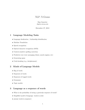
hSihSidogthewalks.hEiFigure 2: Trigram Model for the sentence “the dog walks .” Append special “words” to the sentence– n–1 ‘hSi’ symbols to beginning– only one ‘hEi’ to then end needed p(hEi . hEi) 1.0 since hEi would always be followed by hEi. “the man walks the dog .” (trigrams)– Becomes “hSi hSi the man walks the dog . hEi”– p(hSi hSi the man walks the dog . hEi) p(the hSi hSi)· p(man hSi the)· p(walks the man)· p(the man walks)· p(dog walks the)· p(. the dog)· p(hEi dog .) Can be generalized to model longer texts: paragraphs, documents, etc:– Good: can model ngrams that cross sentences (e.g. p(w0 .) or p(w0 ?))– Bad: more sparsity on hSi and hEi8Sentence Likelihood ExamplesExample dataset: S S S S S S the dog runs . E the dog walks . E the man walks . E a man walks the dog . E the cat walks . E the dog chases the cat . E Sentence Likelihood with Bigrams:p(hSi the dog walks . hEi) p(the hSi) · p(dog the) · p(walks dog) · p(. walks) · p(hEi .)C(hSi the)C(hSi x) P C(hSi the)C(hSi)x V hEi··PC(the dog)x V C(the x)C(the dog)C(the)··C(dog walks)C(dog)PC(dog walks)x V C(dog x)·C(walks .)C(walks)6··P C(walks .)x V C(walks x)C(. hEi)C(.)·PC(. hEi)x V C(. x)
56·47·14·34·66 0.83 · 0.57 · 0.25 · 0.75 · 1.0 0.089p(hSi the cat walks the dog . hEi) p(the hSi) · p(cat the) · p(walks cat) · p(the walks) · p(dog the) · p(. dog) · p(hEi .) PC(hSi the)C(hSi x)x V hEicat)PC(cat walks) · P C(walks the)PC(the dog) · P· P C(theC(thex) ·C(cat x)C(walks x) ·C(the x)x Vx Vx Vx VC(dog .)C(dog x)·x VPC(. hEi)x V C(. x) C(hSi the)C(hSi)·C(the cat)C(the) 5614··17·11·47·14·66·C(cat walks)C(cat)·C(walks the)C(walks)·C(the dog)C(the)·C(dog .)C(dog)·C(. hEi)C(.) 0.83 · 0.14 · 1.0 · 0.25 · 0.57 · 0.25 · 1.0 0.004p(hSi the cat runs . hEi) p(the hSi) · p(cat the) · p(runs cat) · p(. runs) · p(hEi .) P C(hSi the)x V C(hSi x) C(hSi the)C(hSi)·C(the cat)C(the) 5611··17·01··66P C(the cat)x V C(the x)··PC(cat runs)x V C(cat x)C(cat runs)C(cat)·C(runs .)C(runs)··P C(runs .)x V C(runs x)·PC(. hEi)x V C(. x)C(. hEi)C(.) 0.83 · 0.14 · 0.0 · 1.0 · 1.0 0.000 Longer sentences have lower likelihoods.– This makes sense because longer sequences are harder to match exactly. Zeros happen when an n-gram isn’t seen.\\ Day 39Handling SparsityHow big of a problem is sparsity? Alice’s Adventures in Wonderland– Vocabulary (all word types) size: V 3,569– Distinct bigrams: 17,149;– Distinct trigrams: 28,540;17,149, V 217,149, V 3or 99.8% of possible bigrams unseenor 99.9999994% of possible trigrams unseen If a sequence contains an unseen ngram, it will have likelihood zero: an impossible sequence. Many legitimate ngrams will simply be absent from the corpus. This does not mean they are impossible.7
Even ungrammatical/nonsense ngrams should not cause an entire sequence’s likelihood to bezero. Many others will be too infrequent to estimate well.Add-λ Smoothing Add some constant λ to every count, including unseen ngrams V is the Vocabulary — all posslb “next word” types — including hEi (if necessary n 1)– Don’t need hSi because it will never be the ‘next word’ p(w0 w1 n . w 1 ) P C(w1 n . w 1 w0 ) λx V (C(w1 n . w 1 x) λ) P C(w1 n . w 1 w0 ) λ( x V C(w1 n . w 1 x)) λ V C(w1 n . w 1 w0 ) λC(w1 n . w 1 ) λ V – Add V to denominator to account for the fact that there is an extra count for every x In practice it over-smoothes, even when λ 1 Example dataset: S S S S S S S S S S S S the dog runs . E the dog walks . E the man walks . E a man walks the dog . E the cat walks . E the dog chases the cat . E V {a, cat, chases, dog, man, runs, the, walks, ., hEi} V 10Sentence Likelihood with Trigrams:p(“the cat runs .”) p(hSi hSi the cat runs . hEi) p(the hSi hSi) · p(cat hSi the) · p(runs the cat) · p(. cat runs) · p(hEi runs .)C(hSi hSi the)(C(hSi hSi x) 1)P C(runs . hEi) 1x V (C(runs . x) 1) Px V·P C(hSi the cat) 1x V (C(hSi the x) 1) C(hSi hSi the) 1C(hSi hSi) ( V 1)·C(hSi the cat) 1C(hSi the) V 5 16 9·0 10 10·1 15 10·0 12 10···P C(the cat runs) 1x V (C(the cat x) 1)C(the cat runs) 1C(the cat) V ··P C(cat runs .) 1x V (C(cat runs x) 1)C(cat runs .) 1C(cat runs) V ·C(runs . hEi) 1C(runs .) V 1 11 10 0.40 · 0.13 · 0.08 · 0.10 · 0.18 0.000081 If the context was never seen, then the distribution is uniform:C(w 2 w 1 w0 ) λ x V C(w 2 w 1 x) λ · V 0 λ Px V 0 λ · V 0 λλ11 0 λ · V λ · V 1 · V V p λ (w0 w 2 , w 1 ) P8·
Since hSi can never be followed by hEi– p(hEi hSi hSi) 0P– The denominator x V C(hSi hSi x) only gets V -1 smoothing counts hSi not included in V because we can’t transition to it. More smoothing on less common ngrams– With smoothing, we have counts for any possible type following “runs .”:p(hEi runs .) p(the runs .) 1 11 100 11 10 211111 0.18 0.09 Counts of “runs .” are very low (only 1 occurrence), so estimates are bad Bad estimates means more smoothing is good MLE of “runs . hEi” is 1.0, add-1 smoothed becomes 0.18MLE of “runs . the” is 0.0, add-1 smoothed becomes 0.09 Original difference of 1.0 becomes difference of 0.09! This makes sense because our estimates are so bad that we really can’t make ajudgement about what could possibly follow “runs .”– Contexts with higher counts have less smoothing:p(hEi walks .) p(the walks .) 3 13 100 13 10 413113 0.31 0.08 Counts of “walks .” are higher (3 occurrence), so estimates are better Better estimates means less smoothing is good MLE of “walks . hEi” is 1.0, add-1 smoothed becomes 0.31MLE of “walks . the” is 0.0, add-1 smoothed becomes 0.08 Original difference of 1.0 becomes difference of 0.23 Remains a larger gap than we saw for “runs . x” This makes sense because our estimates are better, so we can be more sure that“walks .” should only be followed by hEi Disadvantages of add-λ smoothing:– Over-smoothes.Good-Turing Smoothing Estimate counts of things you haven’t seen from counts of things you have Estimate probability of things which occur c times with the probability of things which occurc 1 times c (c 1) NNc 1cp GT (things with freq 0) pGT (w0 w1 n . w 1 ) N1NC (w1 n . w 1 w0 )C (w1 n . w 1 )9
Knesser-Ney Smoothing Intuition: interpolate based on “openness” of the context Words seen in more contexts are more likely to appear in others Even if we haven’t seen w0 following the context, if the context is “open” (supports a widevariety of “next words”), then it is more likely to support w0 Boost counts based on {x : C(w1 n . w 1 x) 0} , the number of different “next words”seen after w1 n . w 1\\ Day 4Interpolation Mix n-gram probability with probabilities from lower-order modelsp̂(w0 w 2 w 1 ) λ3 · p(w0 w 2 w 1 ) λ2 · p(w0 w 1 ) λ1 · p(w0 ) λi terms used to decide how much to smoothP i λi 1 (still a valid probability distribution, because they are proportions Use dev dataset to tune λ hyperparameters Also useful for combining models trained on different data:– Can interpolate “customized” models with “general” models– Baseline English regional English user-specific English– Little in-domain data, lots of out-of-domainStupid Backoff If p(n-gram) 0, just use p((n-1)-gram) Does not yield a valid probability distribution Works shockingly well for huge datasets10
10Out-of-Vocabulary Words (OOV)Add-λ If ngram contains OOV item, assume count of λ, just like for all other ngrams. Probability distributions become invalid. We can’t know the full vocabulary size, so we can’tnormalize counts correctly.hunki Create special token hunki Create a fixed lexicon L– All types in some subset of training data?– All types appearing more than k times? V L hunki, V L 1 Before training, change any word not in L to hunki Then train as usual as if hunkiwas a normal word For new sentence, again replace words not in L with hunkibefore using model Probabilities containing hunki measure likelihood with some rare word Problem: the “rare” word is no longer rare since there are many hunkitokens– Ngrams with hunkiwill have higher probabilities than those with any particular rareword– Not so bad when comparing same sequence under multiple models. All will have inflatedprobabilities.– More problematic when comparing probabilities of different sequences under the samemodel p(i totes know) p(i totally know) p(i hunki know)11EvaluationExtrinsic Use the model in some larger task. See if it helps. More realistic HarderIntrinsic11
Evaluate on a test corpus EasierPerplexity Intrinsic measure of model quality How well does the model “fit” the test data? How “perplexed” is the model whe it sees the test data? Measure the probability of the test corpus, normalize for number of words.q P P (W ) W p(w1 w2 1. w ) W With individual sentences: P P (s1 , s2 , .) 12qP( i si )Q 1i p(si )Generative Models Generative models are designed to model how the data could have been generated. The best parameters are those that would most likely generate the data. MLE maximizes that likelihood that the training data was generated by the model. As such, we can actually generate data from a model. Trigram model:– General:For each sequence:1. Sample a word w0 according to w0 p(w0 )2. Sample a second word w1 according to w1 p(w1 w0 )3. Sample a next word wk according to wk p(wk wk 2 wk 1 )4. Repeat step 3 until you feel like stopping.– Sentences:For each sentence:1. Sample a word w0 according to w0 p(w0 hSi hSi)2. Sample a second word w1 according to w1 p(w1 w0 hSi)3. Sample a next word wk according to wk p(wk wk 2 wk 1 )4. Repeat until hEi is drawn. Longer n generates more coherent text Too-large n just ends up generating sentences from the training data because most countswill be 1 (no choice of next word). Naı̈ve Bayes was a generative model too!12
nsFigure 3: Finite state machine. Missing arrows are assumed to be zero probabilities. With smoothing, there would be an arrow in both directions between every pair of words.For each instance:1. Sample a label l according to l p(Label l)2. For each feature F : sample a value v according to v p(F v Label l) We will see many more generative models throughout this coursep(S - the) 0.83p(S - a) 0.17p(the - cat) 0.29p(the - dog) 0.57p(the - man) 0.14p(dogp(dogp(dogp(dog- - - - chases) 0.25runs) 0.25.) 0.25walks) 0.25p(chases - the) 1.00p(a - man) 1.00p(runs - .) 1.00p(man - walks) 1.00p(walks - the) 0.25p(walks - .) 0.75p(cat - walks) 0.50p(cat - .) 0.5013p(. - E ) 1.00How much data?Choosing n13
Large n– More context for probabilities:p(phone) vsp(phone cell) vsp(phone your cell) vsp(phone off your cell) vsp(phone turn off your cell)– Long-range dependencies Small n– Better generalization– Better estimates– Long-range dependenciesHow much training data? As much as possible. More data means better estimates Google N-Gram corpus uses 10-grams(a) Data size matters morethan algorithm (Banko and Brill,2001)14(b) Results keep improving withmore data (Norvig: Unreasonable .)(c) With enough data, stupidbackoff approaches Knesser-Neyaccuracy (Brants et al., 2007)CitationsSome content adapted from: http://courses.washington.edu/ling570/gina fall11/slides/ling570 class8 smoothing.pdf14
NLP: N-Grams Dan Garrette dhg@cs.utexas.edu December 27, 2013 1 Language Modeling Tasks Language iden cation / Authorship identi cation Machine Translation Speech recognition Optical character recognition (OCR) Context-sensitive spelling correction Predictive text (text messaging clients, se