WIXLIB

that the data pertains to, and they should be ironed out before valid statistical inference fromsuch data can be produced.Consistent data is the stage where data is ready for statistical inference. It is the data that moststatistical theories use as a starting point. Ideally, such theories can still be applied withouttaking previous data cleaning steps into account. In practice however, data cleaning methodslike imputation of missing values will influence statistical results and so must be accounted for inthe following analyses or interpretation thereof.Once Statistical results have been produced they can be stored for reuse and finally, results canbe Formatted to include in statistical reports or publications.Best practice. Store the input data for each stage (raw, technically correct,consistent, aggregated and formatted) separately for reuse. Each step between thestages may be performed by a separate R script for reproducibility.Summarizing, a statistical analysis can be separated in five stages, from raw data to formattedoutput, where the quality of the data improves in every step towards the final result. Datacleaning encompasses two of the five stages in a statistical analysis, which again emphasizes itsimportance in statistical practice.1.2 Some general background in RWe assume that the reader has some proficiency in R. However, as a service to the reader, belowwe summarize a few concepts which are fundamental to working with R, especially whenworking with dirty data''.1.2.1 Variable types and indexing techniquesIf you had to choose to be proficient in just one R-skill, it should be indexing. By indexing wemean all the methods and tricks in R that allow you to select and manipulate data usinglogical, integer or named indices. Since indexing skills are important for data cleaning, wequickly review vectors, data.frames and indexing techniques.The most basic variable in R is a vector. An R vector is a sequence of values of the same type.All basic operations in R act on vectors (think of the element-wise arithmetic, for example). Thebasic types in R are as eric data (approximations of the real numbers, ℝ)Integer data (whole numbers, ℤ)Categorical data (simple classifications, like gender)Ordinal data (ordered classifications, like educational level)Character data (strings)Binary dataAll basic operations in R work element-wise on vectors where the shortest argument is recycledif necessary. This goes for arithmetic operations (addition, subtraction, ), comparisonoperators ( , , ), logical operators (&, , !, ) and basic math functions like sin, cos, expand so on. If you want to brush up your basic knowledge of vector and recycling properties, youcan execute the following code and think about why it works the way it does.An introduction to data cleaning with R8

# vectors have variables of one typec(1, 2, "three")# shorter arguments are recycled(1:3) * 2(1:4) * c(1, 2)# warning! (why?)(1:4) * (1:3)Each element of a vector can be given a name. This can be done by passing named arguments tothe c() function or later with the names function. Such names can be helpful giving meaning toyour variables. For example compare the vectorx - c("red", "green", "blue")with the one below.capColor c(huey "red", duey "blue", louie "green")Obviously the second version is much more suggestive of its meaning. The names of a vectorneed not be unique, but in most applications you'll want unique names (if any).Elements of a vector can be selected or replaced using the square bracket operator [ ]. Thesquare brackets accept either a vector of names, index numbers, or a logical. In the case of alogical, the index is recycled if it is shorter than the indexed vector. In the case of numericalindices, negative indices omit, in stead of select elements. Negative and positive indices are notallowed in the same index vector. You can repeat a name or an index number, which results inmultiple instances of the same value. You may check the above by predicting and then verifyingthe result of the following or "blue"]x - c(4, 7, 6, 5, 2, 8)I - x 6J - x 7x[I J]x[c(TRUE, FALSE)]x[c(-1, -2)]Replacing values in vectors can be done in the same way. For example, you may check that inthe following assignmentx - 1:10x[c(TRUE, FALSE)] - 1every other value of x is replaced with 1.A list is a generalization of a vector in that it can contain objects of different types, includingother lists. There are two ways to index a list. The single bracket operator always returns asub-list of the indexed list. That is, the resulting type is again a list. The double bracketoperator ([[ ]]) may only result in a single item, and it returns the object in the list itself.Besides indexing, the dollar operator can be used to retrieve a single element. To understandthe above, check the results of the following statements.L - list(x c(1:5), y c("a", "b", "c"), z capColor)L[[2]]L yL[c(1, 3)]L[c("x", "y")]L[["z"]]An introduction to data cleaning with R9

Especially, use the class function to determine the type of the result of each statement.A data.frame is not much more than a list of vectors, possibly of different types, but withevery vector (now columns) of the same length. Since data.frames are a type of list, indexingthem with a single index returns a sub-data.frame; that is, a data.frame with less columns.Likewise, the dollar operator returns a vector, not a sub-data.frame. Rows can be indexedusing two indices in the bracket operator, separated by a comma. The first index indicates rows,the second indicates columns. If one of the indices is left out, no selection is made (soeverything is returned). It is important to realize that the result of a two-index selection issimplified by R as much as possible. Hence, selecting a single column using a two-index resultsin a vector. This behaviour may be switched off using drop FALSE as an extra parameter. Hereare some short examples demonstrating the above.d - data.frame(x 1:10, y letters[1:10], z LETTERS[1:10])d[1]d[, 1]d[, "x", drop FALSE]d[c("x", "z")]d[d x 3, "y", drop FALSE]d[2, ]1.2.2 Special valuesLike most programming languages, R has a number of Special values that are exceptions to thenormal values of a type. These are NA, NULL, Inf and NaN. Below, we quickly illustrate themeaning and differences between them.NA Stands for not available. NA is a placeholder for a missing value. All basic operations in Rhandle NA without crashing and mostly return NA as an answer whenever one of the inputarguments is NA. If you understand NA, you should be able to predict the result of thefollowing R statements.NA 1sum(c(NA, 1, 2))median(c(NA, 1, 2, 3), na.rm TRUE)length(c(NA, 2, 3, 4))3 NANA NATRUE NAThe function is.na can be used to detect NA's.NULL You may think of NULL as the empty set from mathematics. NULL is special since it has noclass (its class is NULL) and has length 0 so it does not take up any space in a vector. Inparticular, if you understand NULL, the result of the following statements should be clear toyou without starting R.length(c(1, 2, NULL, 4))sum(c(1, 2, NULL, 4))x - NULLc(x, 2)The function is.null can be used to detect NULL variables.Inf Stands for infinity and only applies to vectors of class numeric. A vector of class integer cannever be Inf. This is because the Inf in R is directly derived from the international standardfor floating point arithmetic 1 . Technically, Inf is a valid numeric that results fromcalculations like division of a number by zero. Since Inf is a numeric, operations between Infand a finite numeric are well-defined and comparison operators work as expected. If youunderstand Inf, the result of the following statements should be clear to you.An introduction to data cleaning with R10

pi/02 * InfInf - 1e 10Inf Inf3 -InfInf InfNaN Stands for not a number. This is generally the result of a calculation of which the result isunknown, but it is surely not a number. In particular operations like 0/0, Inf-Inf andInf/Inf result in NaN. Technically, NaN is of class numeric, which may seem odd since it isused to indicate that something is not numeric. Computations involving numbers and NaNalways result in NaN, so the result of the following computations should be clear.NaN 1exp(NaN)The function is.nan can be used to detect NaN's.Tip. The function is.finite checks a vector for the occurrence of any non-numericalor special values. Note that it is not useful on character vectors.ExercisesExercise 1.1. Predict the result of the following R statements. Explain the reasoning behind theresults.a.b.c.d.e.exp(-Inf)NA NANA NULLNULL NULLNA & FALSEExercise 1.2. In which of the steps outlined in Figure 1 would you perform the following activities?a.b.c.d.e.Estimating values for empty fields.Setting the font for the title of a histogram.Rewrite a column of categorical variables so that they are all written in capitals.Use the knitr package 38 to produce a statistical report.Exporting data from Excel to csv.An introduction to data cleaning with R11

2 From raw data to technically correct dataA data set is a collection of data that describes attribute values (variables) of a number ofreal-world objects (units). With data that are technically correct, we understand a data set whereeach value1. can be directly recognized as belonging to a certain variable;2. is stored in a data type that represents the value domain of the real-world variable.In other words, for each unit, a text variable should be stored as text, a numeric variable as anumber, and so on, and all this in a format that is consistent across the data set.2.1 Technically correct data in RThe R environment is capable of reading and processing several file and data formats. For thistutorial we will limit ourselves to rectangular' data sets that are to be read from a text-basedformat. In the case of R, we define technically correct data as a data set that– is stored in a data.frame with suitable columns names, and– each column of the data.frame is of the R type that adequately represents the value domainof the variable in the column.The second demand implies that numeric data should be stored as numeric or integer, textualdata should be stored as character and categorical data should be stored as a factor orordered vector, with the appropriate levels.Limiting ourselves to textual data formats for this tutorial may have its drawbacks, but there areseveral favorable properties of textual formats over binary formats:– It is human-readable. When you inspect a text-file, make sure to use a text-reader (more,less) or editor (Notepad, vim) that uses a fixed-width font. Never use an office application forthis purpose since typesetting clutters the data's structure, for example by the use of ligature.– Text is very permissive in the types values that are stored, allowing for comments andannotations.The task then, is to find ways to read a textfile into R and have it transformed to a well-typeddata.frame with suitable column names.Best practice. Whenever you need to read data from a foreign file format, like aspreadsheet or proprietary statistical software that uses undisclosed file formats,make that software responsible for exporting the data to an open format that can beread by R.2.2 Reading text data into a R data.frameIn the following, we assume that the text-files we are reading contain data of at most one unitper line. The number of attributes, their format and separation symbols in lines containing datamay differ over the lines. This includes files in fixed-width or csv-like format, but excludesXML-like storage formats.An introduction to data cleaning with R12

2.2.1 read.table and its cousinsThe following high-level R functions allow you to read in data that is technically correct, or closeto 2read.fwfThe return type of all these functions is a data.frame. If the column names are stored in thefirst line, they can automatically be assigned to the names attribute of the resultingdata.frame.Best practice. A freshly read data.frame should always be inspected with functionslike head, str, and summary.The read.table function is the most flexible function to read tabular data that is stored in atextual format. In fact, the other read-functions mentioned above all eventually useread.table with some fixed parameters and possibly after some preprocessing. 2read.fwffor comma separated values with period as decimal separator.for semicolon separated values with comma as decimal separator.tab-delimited files with period as decimal separator.tab-delimited files with comma as decimal separator.data with a predetermined number of bytes per column.Each of these functions accept, amongst others, the following optional arguments.ArgumentdescriptionDoes the first line contain column names?character vector with column names.Which strings should be considered NA?character vector with the types of columns.Will coerce the columns to the specified types.If TRUE, converts all character vectors intofactor vectors.Field sAsFactorssepUsed only internally by read.fwfExcept for read.table and read.fwf, each of the above functions assumes by default that thefirst line in the text file contains column headers. To demonstrate this, we assume that we havethe following text file stored under files/unnamed.txt.123421,6.042,5.918,5.7*21,NANow consider the following script.An introduction to data cleaning with R13

# first line is erroneously interpreted as column names(person - read.csv("files/unnamed.txt"))##X21 X6.0## 1 42 5.9## 2 18 5.7*## 3 21 NA # so we better do the followingperson - read.csv(file "files/unnamed.txt", header FALSE, col.names c("age","height") )person##age height## 1 216.0## 2 425.9## 3 185.7*## 4 21 NA In the first attempt, read.csv interprets the first line as column headers and fixes the numericdata to meet R's variable naming standards by prepending an X.If colClasses is not specified by the user, read.table will try to determine the column types.Although this may seem convenient, it is noticeably slower for larger files (say, larger than a fewMB) and it may yield unexpected results. For example, in the above script, one of the rowscontains a malformed numerical variable (5.7*), causing R to interpret the whole column as atext variable. Moreover, by default text variables are converted to factor, so we are now stuckwith a height variable expressed as levels in a categorical variable:str(person)## 'data.frame': 4 obs. of 2 variables:## age: int 21 42 18 21## height: Factor w/ 3 levels "5.7*","5.9","6.0": 3 2 1 NAUsing colClasses, we can force R to either interpret the columns in the way we want or throwan error when this is not possible.read.csv("files/unnamed.txt",header FALSE,colClasses c('numeric','numeric'))## Error: scan() expected 'a real', got '5.7*'This behaviour is desirable if you need to be strict about how data is offered to your R script.However, unless you are prepared to write tryCatch constructions, a script containing theabove code will stop executing completely when an error is encountered.As an alternative, columns can be read in as character by setting stringsAsFactors FALSE.Next, one of the as.-functions can be applied to convert to the desired type, as shown below.dat - read.csv(file "files/unnamed.txt", header FALSE, col.names c("age","height"), stringsAsFactors FALSE)dat height - as.numeric(dat height)## Warning: NAs introduced by coercionAn introduction to data cleaning with R14

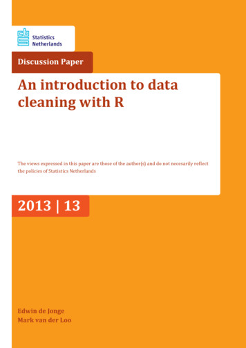
dat##age height## 1 216.0## 2 425.9## 3 18NA## 4 21NANow, everything is read in and the height column is translated to numeric, with the exceptionof the row containing 5.7*. Moreover, since we now get a warning instead of an error, a scriptcontaining this statement will continue to run, albeit with less data to analyse than it wassupposed to. It is of course up to the programmer to check for these extra NA's and handle themappropriately.2.2.2 Reading data with readLinesWhen the rows in a data file are not uniformly formatted you can consider reading in the textline-by-line and transforming the data to a rectangular set yourself. With readLines you canexercise precise control over how each line is interpreted and transformed into fields in arectangular data set. Table 1 gives an overview of the steps to be taken. Below, each step isdiscussed in more detail. As an example we will use a file called daltons.txt. Below, we showthe contents of the file and the actual table with data as it should appear in R.Data file:12345%% Data on the Dalton BrothersGratt ,1861,1892Bob ,18921871,Emmet ,1937% Names, birth and death datesActual 21937The file has comments on several lines (starting with a % sign) and a missing value in the secondrow. Moreover, in the third row the name and birth date have been swapped.Step 1. Reading data. The readLines function accepts filename as argument and returns acharacter vector containing one element for each line in the file. readLines detects both theend-of-line and carriage return characters so lines are detected regardless of whether the filewas created under DOS, UNIX or MAC (each OS has traditionally had different ways of marking anend-of-line). Reading in the Daltons file yields the following.(txt - readLines("files/daltons.txt"))## [1] "%% Data on the Dalton Brothers" "Gratt,1861,1892"## [3] "Bob,1892""1871,Emmet,1937"## [5] "% Names, birth and death dates"The variable txt has 5 elements, equal to the number of lines in the textfile.Step 2. Selecting lines containing data. This is generally done by throwing out lines containingcomments or otherwise lines that do not contain any data fields. You can use grep or grepl todetect such lines.# detect lines starting with a percentage sign.I - grepl(" %", txt)# and throw them out(dat - txt[!I])## [1] "Gratt,1861,1892" "Bob,1892""1871,Emmet,1937"An introduction to data cleaning with R15

Table 1: Steps to take when converting lines in a raw text file to a data.framewith correctly typed columns.123456StepRead the data with readLinesSelect lines containing dataSplit lines into separate fieldsStandardize rowsTransform to data.frameNormalize and coerce to correct typeresultcharactercharacterlist of character vectorslist of equivalent vectorsdata.framedata.frameHere, the first argument of grepl is a search pattern, where the caret (̂) indicates a start-of-line.The result of grepl is a logical vector that indicates which elements of txt contain thepattern 'start-of-line' followed by a percent-sign. The functionality of grep and grepl will bediscussed in more detail in section 2.4.2.Step 3. Split lines into separate fields. This can be done with strsplit. This function acceptsa character vector and a split argument which tells strsplit how to split a string intosubstrings. The result is a list of character vectors.(fieldList - strsplit(dat, split ","))## [[1]]## [1] "Gratt" "1861" "1892"#### [[2]]## [1] "Bob" "1892"#### [[3]]## [1] "1871" "Emmet" "1937"Here, split is a single character or sequence of characters that are to be interpreted as fieldseparators. By default, split is interpreted as a regular expression (see Section 2.4.2) whichmeans you need to be careful when the split argument contains any of the special characterslisted on page 25. The meaning of these special characters can be ignored by passingfixed TRUE as extra parameter.Step 4. Standardize rows. The goal of this step is to make sure that 1) every row has the samenumber of fields and 2) the fields are in the right order. In read.table, lines that contain lessfields than the maximum number of fields detected are appended with NA. One advantage ofthe do-it-yourself approach shown here is that we do not have to make this assumption. Theeasiest way to standardize rows is to write a function that takes a single character vector asinput and assigns the values in the right order.assignFields - function(x

Code.All code examples in this tutorial can be executed, unless otherwise indicated. Code examples are shown in gray boxes, like this: 1 1 ## [1] 2 where output is preceded by a double hash sign##. When code, function names or arguments occur in the main text, these are typeset in fixed widt