Transcription
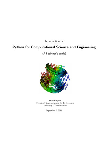
Introduction toPython for Computational Science and Engineering(A beginner’s guide)Hans FangohrFaculty of Engineering and the EnvironmentUniversity of SouthamptonSeptember 7, 2015
2
Contents1 Introduction1.1 Computational Modelling . . . . . . . . . . . . . . . . . .1.1.1 Introduction . . . . . . . . . . . . . . . . . . . . .1.1.2 Computational Modelling . . . . . . . . . . . . . .1.1.3 Programming to support computational modelling1.2 Why Python for scientific computing? . . . . . . . . . . .1.2.1 Optimisation strategies . . . . . . . . . . . . . . .1.2.2 Get it right first, then make it fast . . . . . . . . .1.2.3 Prototyping in Python . . . . . . . . . . . . . . . .1.3 Literature . . . . . . . . . . . . . . . . . . . . . . . . . . .1.3.1 Recorded video lectures on Python for beginners .1.3.2 Python tutor mailing list . . . . . . . . . . . . . .1.4 Python version . . . . . . . . . . . . . . . . . . . . . . . .1.5 This document . . . . . . . . . . . . . . . . . . . . . . . .1.6 Your feedback . . . . . . . . . . . . . . . . . . . . . . . . .999910111213131313141414142 A powerful calculator2.1 Python prompt and Read-Eval-Print Loop (REPL) . .2.2 Calculator . . . . . . . . . . . . . . . . . . . . . . . . .2.3 Integer division . . . . . . . . . . . . . . . . . . . . . .2.3.1 How to avoid integer division . . . . . . . . . .2.3.2 Why should I care about this division problem?2.4 Mathematical functions . . . . . . . . . . . . . . . . .2.5 Variables . . . . . . . . . . . . . . . . . . . . . . . . .2.5.1 Terminology . . . . . . . . . . . . . . . . . . .2.6 Impossible equations . . . . . . . . . . . . . . . . . . .2.6.1 The notation . . . . . . . . . . . . . . . . .17171718181920212222233 Data Types and Data Structures3.1 What type is it? . . . . . . . . .3.2 Numbers . . . . . . . . . . . . . .3.2.1 Integers . . . . . . . . . .3.2.2 Long integers . . . . . . .3.2.3 Floating Point numbers .3.2.4 Complex numbers . . . .3.2.5 Functions applicable to all3.3 Sequences . . . . . . . . . . . . .3.3.1 Sequence type 1: String .3.3.2 Sequence type 2: List . .3.3.3 Sequence type 3: Tuples .252525252626272727282931. . . . . . . . . . . . . . . . . . . . . . . . .types of. . . . . . . . . . . . . . . . .3. . . . . . . . . . . . . . . . . . . . . . . . . . . . . . .numbers . . . . . . . . . . . . . . . . . . . . .
4CONTENTS3.43.53.3.4 Indexing sequences . . . . . . . .3.3.5 Slicing sequences . . . . . . . . .3.3.6 Dictionaries . . . . . . . . . . . .Passing arguments to functions . . . . .3.4.1 Call by value . . . . . . . . . . .3.4.2 Call by reference . . . . . . . . .3.4.3 Argument passing in Python . .3.4.4 Performance considerations . . .3.4.5 Inadvertent modification of data3.4.6 Copying objects . . . . . . . . .Equality and Identity/Sameness . . . . .3.5.1 Equality . . . . . . . . . . . . . .3.5.2 Identity / Sameness . . . . . . .3.5.3 Example: Equality and identity .4 Introspection4.1 dir() . . . . . . . . .4.1.1 Magic names4.2 type . . . . . . . . .4.3 isinstance . . . . . .4.4 help . . . . . . . . .4.5 Docstrings . . . . . .3233353737383940414242424343.454546464747495 Input and Output5.1 Printing to standard output (normally the screen) . . . . . . . . .5.1.1 Simple print (not compatible with Python 3.x) . . . . . . .5.1.2 Formatted printing . . . . . . . . . . . . . . . . . . . . . . .5.1.3 “str” and “ str ” . . . . . . . . . . . . . . . . . . . . . . .5.1.4 “repr” and “ repr ” . . . . . . . . . . . . . . . . . . . . . .5.1.5 Changes from Python 2 to Python 3: print . . . . . . . . .5.1.6 Changes from Python 2 to Python 3: formatting of strings5.2 Reading and writing files . . . . . . . . . . . . . . . . . . . . . . . .5.2.1 File reading examples . . . . . . . . . . . . . . . . . . . . .515151525353545455566 Control Flow6.1 Basics . . . . . . . . . . . . . . . . . . .6.1.1 Conditionals . . . . . . . . . . .6.2 If-then-else . . . . . . . . . . . . . . . .6.3 For loop . . . . . . . . . . . . . . . . . .6.4 While loop . . . . . . . . . . . . . . . .6.5 Relational operators (comparisons) in if6.6 Exceptions . . . . . . . . . . . . . . . .6.6.1 Raising Exceptions . . . . . . . .6.6.2 Creating our own exceptions . .6.6.3 LBYL vs EAFP . . . . . . . . . . . . . . . . . . . . . . . . . . . . . . . . . . . . . . . . . . . . . . . . . . . . . . . . . . . . . . . . . . . . .and while statements. . . . . . . . . . . . . . . . . . . . . . . . . . . . . . . . . . . . . . . . . . . . . . . . .59595961616262636465657 Functions and modules7.1 Introduction . . . . . . . . . . . . . . . .7.2 Using functions . . . . . . . . . . . . . .7.3 Defining functions . . . . . . . . . . . .7.4 Default values and optional parameters.6767676870.
CONTENTS7.5Modules . . . . . . . . . .7.5.1 Importing modules7.5.2 Creating modules .7.5.3 Use of name . .7.5.4 Example 1 . . . . .7.5.5 Example 2 . . . . .5.717172737374.77777878798082839 Common tasks9.1 Many ways to compute a series . . . . . . . . . . . . . . . . . . . . . . . . . . . . . . .9.2 Sorting . . . . . . . . . . . . . . . . . . . . . . . . . . . . . . . . . . . . . . . . . . . . .85858810 From Matlab to Python10.1 Important commands . . . .10.1.1 The for-loop . . . . .10.1.2 The if-then statement10.1.3 Indexing . . . . . . . .10.1.4 Matrices . . . . . . . .9191919191928 Functional tools8.1 Anonymous functions . . .8.2 Map . . . . . . . . . . . . .8.3 Filter . . . . . . . . . . . .8.4 List comprehension . . . . .8.5 Reduce . . . . . . . . . . . .8.6 Why not just use for-loops?8.7 Speed . . . . . . . . . . . .11 Python shells11.1 IDLE . . . . . . . . . . . . .11.2 Python (command line) . . .11.3 Interactive Python (IPython)11.3.1 IPython console . . .11.3.2 IPython Notebook . .11.4 Spyder . . . . . . . . . . . . .11.5 Editors . . . . . . . . . . . . .939393939394959512 Symbolic computation12.1 SymPy . . . . . . . . . . . . . . . . . . . . . . . . .12.1.1 Symbols . . . . . . . . . . . . . . . . . . . .12.1.2 isympy . . . . . . . . . . . . . . . . . . . . .12.1.3 Numeric types . . . . . . . . . . . . . . . .12.1.4 Differentiation and Integration . . . . . . .12.1.5 Ordinary differential equations . . . . . . .12.1.6 Series expansions and plotting . . . . . . .12.1.7 Linear equations and matrix inversion . . .12.1.8 Non linear equations . . . . . . . . . . . . .12.1.9 Output: LATEX interface and pretty-printing12.1.10 Automatic generation of C code . . . . . .12.2 Related tools . . . . . . . . . . . . . . . . . . . . .979797989999101103104106107108109.
6CONTENTS13 Numerical Computation13.1 Numbers and numbers . . . . . . . . . . . . . . .13.1.1 Limitations of number types . . . . . . .13.1.2 Using floating point numbers (carelessly)13.1.3 Using floating point numbers carefully 1 .13.1.4 Using floating point numbers carefully 2 .13.1.5 Symbolic calculation . . . . . . . . . . . .13.1.6 Summary . . . . . . . . . . . . . . . . . .13.1.7 Exercise: infinite or finite loop . . . . . .11111111111311411411511611714 Numerical Python (numpy): arrays14.1 Numpy introduction . . . . . . . . . . . . .14.1.1 History . . . . . . . . . . . . . . . .14.1.2 Arrays . . . . . . . . . . . . . . . . .14.1.3 Convert from array to list or tuple .14.1.4 Standard Linear Algebra operations14.1.5 More numpy examples. . . . . . . . .14.1.6 Numpy for Matlab users . . . . . . 45147147147148148.15 Visualising Data15.1 Matplotlib (Pylab) – plotting y f(x), (and a bit more) . . .15.1.1 Matplotlib and Pylab . . . . . . . . . . . . . . . . .15.1.2 First example . . . . . . . . . . . . . . . . . . . . . .15.1.3 How to import matplotlib, pylab, pyplot, numpy and15.1.4 IPython’s inline mode . . . . . . . . . . . . . . . . .15.1.5 Saving the figure to a file . . . . . . . . . . . . . . .15.1.6 Interactive mode . . . . . . . . . . . . . . . . . . . .15.1.7 Fine tuning your plot . . . . . . . . . . . . . . . . .15.1.8 Plotting more than one curve . . . . . . . . . . . . .15.1.9 Histograms . . . . . . . . . . . . . . . . . . . . . . .15.1.10 Visualising matrix data . . . . . . . . . . . . . . . .15.1.11 Plots of z f (x, y) and other features of Matplotlib15.2 Visual Python . . . . . . . . . . . . . . . . . . . . . . . . . .15.2.1 Basics, rotating and zooming . . . . . . . . . . . . .15.2.2 Setting the frame rate for animations . . . . . . . .15.2.3 Tracking trajectories . . . . . . . . . . . . . . . . . .15.2.4 Connecting objects (Cylinders, springs, . . . ) . . . . .15.2.5 3d vision . . . . . . . . . . . . . . . . . . . . . . . .15.3 Visualising higher dimensional data . . . . . . . . . . . . . .15.3.1 Mayavi, Paraview, Visit . . . . . . . . . . . . . . . .15.3.2 Writing vtk files from Python (pyvtk) . . . . . . . .16 Numerical Methods using Python (scipy)16.1 Overview . . . . . . . . . . . . . . . . . .16.2 SciPy . . . . . . . . . . . . . . . . . . . .16.3 Numerical integration . . . . . . . . . . .16.3.1 Exercise: integrate a function . . .16.3.2 Exercise: plot before you integrate16.4 Solving ordinary differential equations . .16.4.1 Exercise: using odeint . . . . . . . . . .all. . . . . . . . . . . . . . . . . . . . . . . .that. . . . . . . . . . . . . . . . . . . . . . . . . . . . . . . . . . .
CONTENTS716.5 Root finding . . . . . . . . . . . . . . . . . . . . . . . .16.5.1 Root finding using the bisection method . . . .16.5.2 Exercise: root finding using the bisect method16.5.3 Root finding using the fsolve funcion . . . . .16.6 Interpolation . . . . . . . . . . . . . . . . . . . . . . .16.7 Curve fitting . . . . . . . . . . . . . . . . . . . . . . .16.8 Fourier transforms . . . . . . . . . . . . . . . . . . . .16.9 Optimisation . . . . . . . . . . . . . . . . . . . . . . .16.10Other numerical methods . . . . . . . . . . . . . . . .16.11scipy.io: Scipy-input output . . . . . . . . . . . . . . .17 Where to go from here?17.1 Advanced programming . . . . . . . .17.2 Compiled programming language . . .17.3 Testing . . . . . . . . . . . . . . . . .17.4 Simulation models . . . . . . . . . . .17.5 Software engineering for research codes17.6 Data and visualisation . . . . . . . . .17.7 Version control . . . . . . . . . . . . .17.8 Parallel execution . . . . . . . . . . . 166166166
8CONTENTS
Chapter 1IntroductionThis text summarises a number of core ideas relevant to Computational Engineering and ScientificComputing using Python. The emphasis is on introducing some basic Python (programming) conceptsthat are relevant for numerical algorithms. The later chapters touch upon numerical libraries suchas numpy and scipy each of which deserves much more space than provided here. We aim to enablethe reader to learn independently how to use other functionality of these libraries using the availabledocumentation (online and through the packages itself).1.11.1.1Computational ModellingIntroductionIncreasingly, processes and systems are researched or developed through computer simulations: newaircraft prototypes such as for the recent A380 are first designed and tested virtually through computersimulations. With the ever increasing computational power available through supercomputers, clustersof computers and even desktop and laptop machines, this trend is likely to continue.Computer simulations are routinely used in fundamental research to help understand experimentalmeasurements, and to replace – for example – growth and fabrication of expensive samples/experimentswhere possible. In an industrial context, product and device design can often be done much morecost effectively if carried out virtually through simulation rather than through building and testingprototypes. This is in particular so in areas where samples are expensive such as nanoscience (where itis expensive to create small things) and aerospace industry (where it is expensive to build large things).There are also situations where certain experiments can only be carried out virtually (ranging fromastrophysics to study of effects of large scale nuclear or chemical accidents). Computational modelling,including use of computational tools to post-process, analyse and visualise data, has been used inengineering, physics and chemistry for many decades but is becoming more important due to thecheap availability of computational resources. Computational Modelling is also starting to play amore important role in studies of biological systems, the economy, archeology, medicine, health care,and many other domains.1.1.2Computational ModellingTo study a process with a computer simulation we distinguish two steps: the first one is to develop amodel of the real system. When studying the motion of a small object, such as a penny, say, under theinfluence of gravity, we may be able to ignore friction of air: our model — which might only considerthe gravitational force and the penny’s inertia, i.e. a(t) F/m 9.81m/s2 — is an approximationof the real system. The model will normally allow us to express the behaviour of the system (in9
10CHAPTER 1. INTRODUCTIONsome approximated form) through mathematical equations, which often involve ordinary differentialequations (ODEs) or partial differential equatons (PDEs).In the natural sciences such as physics, chemistry and related engineering, it is often not so difficultto find a suitable model, although the resulting equations tend to be very difficult to solve, and canin most cases not be solved analytically at all.On the other hand, in subjects that are not as well described through a mathematical frameworkand depend on behaviour of objects whose actions are impossible to predict deterministically (suchas humans), it is much more difficult to find a good model to describe reality. As a rule of thumb,in these disciplines the resulting equations are easier to solve, but they are harder to find and thevalidity of a model needs to be questioned much more. Typical examples are attempts to simulate theeconomy, the use of global resources, the behaviour of a panicking crowd, etc.So far, we have just discussed the development of models to describe reality, and using these modelsdoes not necessarily involve any computers or numerical work at all. In fact, if a model’s equation canbe solved analytically, then one should do this and write down the solution to the equation.In practice, hardly any model equations of systems of interest can be solved analytically, and thisis where the computer comes in: using numerical methods, we can at least study the model for aparticular set of boundary conditions. For the example considered above, we may not be able to easilysee from a numerical solution that the penny’s velocity under the influence of gravity will changelinearly with time (which we can read easily from the analytical solution that is available for thissimple system: v(t) t · 9.81m/s2 v0 ).The numerical solution that can be computed using a computer would consist of data that showshow the velocity changes over time for a particular initial velocity v0 (v0 is a boundary condition here).The computer program would report a long lists of two numbers keeping the (i) value of time ti forwhich a particular (ii) value of the velocity vi has been computed. By plotting all vi against ti , or byfitting a curve through the data, we may be able to understand the trend from the data (which wecan just see from the analytical solution of course).It is clearly desirable to find an analytical solutions wherever possible but the number of problemswhere this is possible is small. Usually, the obtaining numerical result of a computer simulation is veryuseful (despite the shortcomings of the numerical results in comparison to an analytical expression)because it is the only possible way to study the system at all.The name computational modelling derives from the two steps: (i) modelling, i.e. finding a modeldescription of a real system, and (ii) solving the resulting model equations using computational methods because this is the only way the equations can be solved at all.1.1.3Programming to support computational modellingA large number of packages exist that provide computational modelling capabilities. If these satisfy theresearch or design needs, and any data processing and visualisation is appropriately supported throughexisting tools, one can carry out computational modelling studies without any deeper programmingknowledge.In a research environment – both in academia and research on new products/ideas/. in industry– one often reaches a point where existing packages will not be able to perform a required simulationtask, or where more can be learned from analysing existing data in news ways etc.At that point, programming skills are required. It is also generally useful to have a broad understanding of the building blocks of software and basic ideas of software engineering as we use more andmore devices that are software-controlled.It is often forgotten that there is nothing the computer can do that we as humans cannot do. Thecomputer can do it much faster, though, and also with making far fewer mistakes. There is thus nomagic in computations a computer carries out: they could have been done by humans, and – in fact– were for many years (see for example Wikipedia entry on Human Computer).
1.2. WHY PYTHON FOR SCIENTIFIC COMPUTING?11Understanding how to build a computer simulation comes roughly down to: (i) finding the model(often this means finding the right equations), (ii) knowing how to solve these equations numerically,(ii) to implement the methods to compute these solutions (this is the programming bit).1.2Why Python for scientific computing?The design focus on the Python language is on productivity and code readability, for example through: Interactive python console Very clear, readable syntax through whitespace indentation Strong introspection capabilities Full modularity, supporting hierarchical packages Exception-based error handling Dynamic data types & automatic memory managementAs Python is an interpreted language, and it runs many times slower than compiled code, one mightask why anybody should consider such a ’slow’ language for computer simulations?There are two replies to this criticism:1. Implementation time versus execution time: It is not the execution time alone that contributesto the cost of a computational project: one also needs to consider the cost of the developmentand maintenance work.In the early days of scientific computing (say in the 1960/70/80), compute time was so expensivethat it made perfect sense to invest many person months of a programmer’s time to improve theperformance of a calculation by a few percent.Nowadays, however, the CPU cycles have become much cheaper than the programmer’s time.For research codes which often run only a small number of times (before the researchers moveon to the next problem), it may be economic to accept that the code runs only at 25% of theexpected possible speed if this saves, say, a month of a researcher’s (or programmers) time. Forexample: if the execution time of the piece of code is 10 hours, and one can predict that it willrun about 100 times, then the total execution time is approximately 1000 hours. It would begreat if this could be reduced to 25% and one could save 750 (CPU) hours. On the other hand,is an extra wait (about a month) and the cost of 750 CPU hours worth investing one month of aperson’s time [who could do something else while the calculation is running]? Often, the answeris not.Code readability & maintenance - short code, fewer bugs: A related issue is that a research codeis not only used for one project, but carries on to be used again and again, evolves, grows,bifurcates etc. In this case, it is often justified to invest more time to make the code fast. Atthe same time, a significant amount of programmer time will go into (i) introducing the requiredchanges, (ii) testing them even before work on speed optimisation of the changed version canstart. To be able to maintain, extend and modify a code in often unforeseen ways, it can onlybe helpful to use a language that is easy to read and of great expressive power.
12CHAPTER 1. INTRODUCTION2. Well-written Python code can be very fast if time critical parts in executed through compiledlanguage.Typically, less than 5% percent of the code base of a simulation project need more than 95% ofthe execution time. As long as these calculations are done very efficiently, one doesn’t need toworry about all other parts of the code as the overall time their execution takes is insignificant.The compute intense part of the program should to be tuned to reach optimal performance.Python offers a number of options. For example, the numpy Python extension provides a Python interface to the compiled andefficient LAPACK libraries that are the quasi-standard in numerical linear algebra. If theproblems under study can be formulated such that eventually large systems of algebraicequations have to be solved, or eigenvalues computed, etc, then the compiled code in theLAPACK library can be used (through the Python-numpy package). At this stage, thecalculations are carried out with the same performance of Fortran/C as it is essentiallyFortran/C code that is used. Matlab, by the way, exploits exactly this: the Matlab scriptinglanguage is very slow (about 10 time slower than Python), but Matlab gains its power fromdelegating the matix operation to the compiled LAPACK libraries. Existing numerical C/Fortran libraries can be interfaced to be usable from within Python(using for example Swig, Boost.Python and Cython). Python can be extended through compiled languages if the computationally demandingpart of the problem is algorithmically non-standard and no existing libraries can be used.Commonly used are C, Fortran and C to implement fast extensions. We list some tools that are used to use compiled code from Python:. The scipy.weave extension is useful if just a short expression needs to be expressedin C. The Cython interface is growing in popularity to (i) semi-automatically declare variabletypes in Python code, to translate that code to C (automatically) and to then use thecompiled C code from Python. Cython is also used to quickly wrap an existing Clibrary with an interface so the C library can be used from Python. Boost.Python is specialised for wrapping C code in Python.The conclusion is that Python is ”fast enough” for most computational tasks, and that its user friendlyhigh-level language often makes up for reduced speed in comparison to compiled lower-level languages.Combining Python with tailor-written compiled code for the performance critical parts of the code,results in virtually optimal speed in most cases.1.2.1Optimisation strategiesWe generally understand reduction of execution time when discussing “code optimisation” in thecontext of computational modelling, and we essentially like to carry out the required calculations asfast as possible. (Sometimes we need to reduce the amount of RAM, the amount of data input outputto disk or the network.) At the same time, we need to make sure that we do not invest inappropriateamounts of programming time to achieve this speed up: as always there needs to be a balance betweenthe programmers’ time and the improvement we can gain from this.
1.3. LITERATURE1.2.213Get it right first, then make it fastTo write fast code effectively, we note that the right order is to (i) first write a program that carriesout the correct calculation. For this, choose a language/approach that allows you to write the codequickly and make it work quickly — regardless of execution speed. Then (ii) either change the programor re-write it from scratch in the same language to make the execution faster. During the process,keep comparing results with the slow version written first to make sure the optimisation does notintroduce errors. (Once we are familiar with the concept of regression tests, they should be used hereto compare the new and hopefully faster code with the original code.)A common pattern in Python is to start writing pure Python code, then start using Python librariesthat use compiled code internally (such as the fast arrays Numpy provides, and routines from scipythat go back to established numerical codes such as ODEPACK, LAPACK and others). If required,one can – after careful profiling – start to replace parts of the Python code with a compiled languagesuch as C and Fortran to improve execution speed further (as discussed above).1.2.3Prototyping in PythonIt turns out that – even if a particular code has to be written in, say, C – it is (often) more timeefficient to prototype the code in Python, and once an appropriate design (and class structure) hasbeen found, to translate the code to C .1.3LiteratureWhile this text starts with an introduction of (some aspects of) the basic Python programminglanguage, you may find - depending on your prior experience - that you need to refer to secondarysources to fully understand some ideas.We repeatedly refer to the following documents: Allen Downey, Think Python. Available online in html and pdf thon.html, or from Amazon. The Python documentation http://www.python.org/doc/, and: The Python tutorial (http://docs.python.org/tutorial/)You may also find the following links useful: The numpy home page (http://numpy.scipy.org/) The scipy home page (http://scipy.org/) The matplotlib home page (http://matplotlib.sourceforge.net/). The Python style guide rded video lectures on Python for beginnersDo you like to listen/follow lectures? There is a series of 24 lectures titled Introduction to ComputerScience and Programming delivered by Eric Grimsom and John Guttag from the MIT available erscience-and-programming-fall-2008/ This is aimed at students with little or no programming experience. It aims to provide students with an understanding of the role computation can play in solvingproblems. It also aims to help stude
Introduction to Python for Computational Science and Engineering (A beginner’s guide) Hans Fangohr Faculty of
