WIXLIB

VersionRelease Date0.12.02013-07-23ExamplesInstallation or SetupDetailed instructions on getting pandas set up or installed can be found here in the officialdocumentation.Installing pandas with AnacondaInstalling pandas and the rest of the NumPy and SciPy stack can be a little difficult forinexperienced users.The simplest way to install not only pandas, but Python and the most popular packages that makeup the SciPy stack (IPython, NumPy, Matplotlib, .) is with Anaconda, a cross-platform (Linux,Mac OS X, Windows) Python distribution for data analytics and scientific computing.After running a simple installer, the user will have access to pandas and the rest of the SciPy stackwithout needing to install anything else, and without needing to wait for any software to becompiled.Installation instructions for Anaconda can be found here.A full list of the packages available as part of the Anaconda distribution can be found here.An additional advantage of installing with Anaconda is that you don’t require admin rights to installit, it will install in the user’s home directory, and this also makes it trivial to delete Anaconda at alater date (just delete that folder).Installing pandas with MinicondaThe previous section outlined how to get pandas installed as part of the Anaconda distribution.However this approach means you will install well over one hundred packages and involvesdownloading the installer which is a few hundred megabytes in size.If you want to have more control on which packages, or have a limited internet bandwidth, theninstalling pandas with Miniconda may be a better solution.Conda is the package manager that the Anaconda distribution is built upon. It is a packagemanager that is both cross-platform and language agnostic (it can play a similar role to a pip andvirtualenv combination).Miniconda allows you to create a minimal self contained Python installation, and then use theConda command to install additional packages.First you will need Conda to be installed and downloading and running the Miniconda will do thishttps://riptutorial.com/3

for you. The installer can be found here.The next step is to create a new conda environment (these are analogous to a virtualenv but theyalso allow you to specify precisely which Python version to install also). Run the followingcommands from a terminal window:conda create -n name of my env pythonThis will create a minimal environment with only Python installed in it. To put your self inside thisenvironment run:source activate name of my envOn Windows the command is:activate name of my envThe final step required is to install pandas. This can be done with the following command:conda install pandasTo install a specific pandas version:conda install pandas 0.13.1To install other packages, IPython for example:conda install ipythonTo install the full Anaconda distribution:conda install anacondaIf you require any packages that are available to pip but not conda, simply install pip, and use pipto install these packages:conda install pippip install djangoUsually, you would install pandas with one of packet managers.pip example:pip install pandasThis will likely require the installation of a number of dependencies, including NumPy, will require acompiler to compile required bits of code, and can take a few minutes to complete.https://riptutorial.com/4

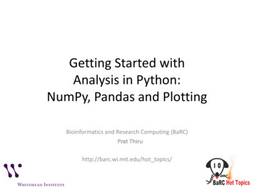
Install via anacondaFirst download anaconda from the Continuum site. Either via the graphical installer(Windows/OSX) or running a shell script (OSX/Linux). This includes pandas!If you don't want the 150 packages conveniently bundled in anaconda, you can install miniconda.Either via the graphical installer (Windows) or shell script (OSX/Linux).Install pandas on miniconda using:conda install pandasTo update pandas to the latest version in anaconda or miniconda use:conda update pandasHello WorldOnce Pandas has been installed, you can check if it is is working properly by creating a dataset ofrandomly distributed values and plotting its histogram.import pandas as pd # This is always assumed but is included here as an introduction.import numpy as npimport matplotlib.pyplot as pltnp.random.seed(0)values np.random.randn(100) # array of normally distributed random numberss pd.Series(values) # generate a pandas seriess.plot(kind 'hist', title 'Normally distributed random values') # hist computes distributionplt.show()https://riptutorial.com/5

Check some of the data's statistics (mean, standard deviation, etc.)s.describe()# Output: count100.000000# mean0.059808# std1.012960# min-2.552990# 25%-0.643857# 50%0.094096# 75%0.737077# max2.269755# dtype: float64Descriptive statisticsDescriptive statistics (mean, standard deviation, number of observations, minimum, maximum,and quartiles) of numerical columns can be calculated using the .describe() method, which returnsa pandas dataframe of descriptive statistics.In [1]: df pd.DataFrame({'A': [1, 2, 1, 4, 3, 5, 2, 3, 4, 1],'B': [12, 14, 11, 16, 18, 18, 22, 13, 21, 17],'C': ['a', 'a', 'b', 'a', 'b', 'c', 'b', 'a', 'b', 'a']})In [2]: dfOut[2]:AB C0 1 12 ahttps://riptutorial.com/6

123456789214352341141116181822132117ababcbabaIn [3]: df.describe()Out[3]:ABcount 10.000000 10.000000mean2.600000 16.200000std1.4298413.705851min1.000000 11.00000025%1.250000 13.25000050%2.500000 16.50000075%3.750000 18.000000max5.000000 22.000000Note that since C is not a numerical column, it is excluded from the output.In [4]: df['C'].describe()Out[4]:count10unique3freq5Name: C, dtype: objectIn this case the method summarizes categorical data by number of observations, number ofunique elements, mode, and frequency of the mode.Read Getting started with pandas online: tartedwith-pandashttps://riptutorial.com/7

Chapter 2: Analysis: Bringing it all togetherand making decisionsExamplesQuintile Analysis: with random dataQuintile analysis is a common framework for evaluating the efficacy of security factors.What is a factorA factor is a method for scoring/ranking sets of securities. For a particular point in time and for aparticular set of securities, a factor can be represented as a pandas series where the index is anarray of the security identifiers and the values are the scores or ranks.If we take factor scores over time, we can, at each point in time, split the set of securities into 5equal buckets, or quintiles, based on the order of the factor scores. There is nothing particularlysacred about the number 5. We could have used 3 or 10. But we use 5 often. Finally, we track theperformance of each of the five buckets to determine if there is a meaningful difference in thereturns. We tend to focus more intently on the difference in returns of the bucket with the highestrank relative to that of the lowest rank.Let's start by setting some parameters and generating random data.To facilitate the experimentation with the mechanics, we provide simple code to create randomdata to give us an idea how this works.Random Data Includes Returns: generate random returns for specified number of securities and periods. Signals: generate random signals for specified number of securities and periods and withprescribed level of correlation with Returns. In order for a factor to be useful, there must besome information or correlation between the scores/ranks and subsequent returns. If thereweren't correlation, we would see it. That would be a good exercise for the reader, duplicatethis analysis with random data generated with 0 correlation.Initializationimport pandas as pdimport numpy as npnum securities 1000num periods 1000period frequency 'W'https://riptutorial.com/8

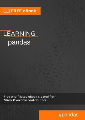
start date '2000-12-31'np.random.seed([3,1415])means [0, 0]covariance [[ 1., 5e-3],[5e-3,1.]]# generates to sets of data m[0] and m[1] with 0.005 correlationm np.random.multivariate normal(means, covariance,(num periods, num securities)).TLet's now generate a time series index and an index representing security ids. Then use them tocreate dataframes for returns and signalsids pd.Index(['s{:05d}'.format(s) for s in range(num securities)], 'ID')tidx pd.date range(start start date, periods num periods, freq period frequency)I divide m[0] by 25 to scale down to something that looks like stock returns. I also add 1e-7 to give amodest positive mean return.security returns pd.DataFrame(m[0] / 25 1e-7, tidx, ids)security signals pd.DataFrame(m[1], tidx, ids)pd.qcut- Create Quintile BucketsLet's use pd.qcut to divide my signals into quintile buckets for each period.def qcut(s, q 5):labels ['q{}'.format(i) for i in range(1, 6)]return pd.qcut(s, q, labels labels)cut security signals.stack().groupby(level 0).apply(qcut)Use these cuts as an index on our returnsreturns cut security returns.stack().rename('returns') \.to frame().set index(cut, append True) \.swaplevel(2, 1).sort index().squeeze() \.groupby(level [0, 1]).mean().unstack()AnalysisPlot Returnsimport matplotlib.pyplot as pltfig plt.figure(figsize (15, 5))https://riptutorial.com/9

ax1 plt.subplot2grid((1,3), (0,0))ax2 plt.subplot2grid((1,3), (0,1))ax3 plt.subplot2grid((1,3), (0,2))# Cumulative Returnsreturns cut.add(1).cumprod() \.plot(colormap 'jet', ax ax1, title "Cumulative Returns")leg1 ax1.legend(loc 'upper left', ncol 2, prop {'size': 10}, fancybox True)leg1.get frame().set alpha(.8)# Rolling 50 Week Returnreturns cut.add(1).rolling(50).apply(lambda x: x.prod()) \.plot(colormap 'jet', ax ax2, title "Rolling 50 Week Return")leg2 ax2.legend(loc 'upper left', ncol 2, prop {'size': 10}, fancybox True)leg2.get frame().set alpha(.8)# Return Distributionreturns cut.plot.box(vert False, ax ax3, title "Return Distribution")fig.autofmt xdate()plt.show()Visualize Quintile Correlation with scatter matrixfrom pandas.tools.plotting import scatter matrixscatter matrix(returns cut, alpha 0.5, figsize (8, 8), diagonal 'hist')plt.show()https://riptutorial.com/10

Calculate and visualize Maximum Draw Downdef max dd(returns):"""returns is a series"""r returns.add(1).cumprod()dd r.div(r.cummax()).sub(1)mdd dd.min()end dd.argmin()start r.loc[:end].argmax()return mdd, start, enddef max dd df(returns):"""returns is a dataframe"""series lambda x: pd.Series(x, ['Draw Down', 'Start', 'End'])return returns.apply(max dd).apply(series)What does this look likemax dd df(returns cut)https://riptutorial.com/11

Let's plot itdraw downs max dd df(returns cut)fig, axes plt.subplots(5, 1, figsize (10, 8))for i, ax in enumerate(axes[::-1]):returns cut.iloc[:, i].add(1).cumprod().plot(ax ax)sd, ed draw downs[['Start', 'End']].iloc[i]ax.axvspan(sd, ed, alpha 0.1, color 'r')ax.set ylabel(returns cut.columns[i])fig.suptitle('Maximum Draw Down', fontsize 18)fig.tight layout()plt.subplots adjust(top .95)https://riptutorial.com/12

Calculate StatisticsThere are many potential statistics we can include. Below are just a few, but demonstrate howsimply we can incorporate new statistics into our summary.def frequency of time series(df):start, end df.index.min(), df.index.max()delta end - startreturn round((len(df) - 1.) * 365.25 / delta.days, 2)def annualized return(df):freq frequency of time series(df)return df.add(1).prod() ** (1 / freq) - 1def annualized volatility(df):freq frequency of time series(df)return df.std().mul(freq ** .5)def sharpe ratio(df):return annualized return(df) / annualized volatility(df)def describe(df):https://riptutorial.com/13

r annualized return(df).rename('Return')v annualized volatility(df).rename('Volatility')s sharpe ratio(df).rename('Sharpe')skew df.skew().rename('Skew')kurt df.kurt().rename('Kurtosis')desc df.describe().Treturn pd.concat([r, v, s, skew, kurt, desc], axis 1).T.drop('count')We'll end up using just the describe function as it pulls all the others together.describe(returns cut)This is not meant to be comprehensive. It's meant to bring many of pandas' features together anddemonstrate how you can use it to help answer questions important to you. This is a subset of thetypes of metrics I use to evaluate the efficacy of quantitative factors.Read Analysis: Bringing it all together and making decisions ionshttps://riptutorial.com/14

Chapter 3: Appending to DataFrameExamplesAppending a new row to DataFrameIn [1]: import pandas as pdIn [2]: df pd.DataFrame(columns ['A', 'B', 'C'])In [3]: dfOut[3]:Empty DataFrameColumns: [A, B, C]Index: []Appending a row by a single column value:In [4]: df.loc[0, 'A'] 1In [5]: dfOut[5]:ABC0 1 NaN NaNAppending a row, given list of values:In [6]: df.loc[1] [2, 3, 4]In [7]: dfOut[7]:ABC0 1 NaN NaN1 234Appending a row given a dictionary:In [8]: df.loc[2] {'A': 3, 'C': 9, 'B': 9}In [9]: dfOut[9]:ABC0 1 NaN NaN1 2342 399The first input in .loc[] is the index. If you use an existing index, you will overwrite the values in thatrow:In [17]: df.loc[1] [5, 6, 7]https://riptutorial.com/15

In [18]: dfOut[18]:ABC0 1 NaN NaN1 5672 399In [19]: df.loc[0, 'B'] 8In [20]: dfOut[20]:A BC0 1 8 NaN1 5 672 3 99Append a DataFrame to another DataFrameLet us assume we have the following two DataFrames:In [7]: df1Out[7]:AB0 a1 b11 a2 b2In [8]: df2Out[8]:BC0 b1 c1The two DataFrames are not required to have the same set of columns. The append method doesnot change either of the original DataFrames. Instead, it returns a new DataFrame by appendingthe original two. Appending a DataFrame to another one is quite simple:In [9]:Out[9]:A0a11a20 NaNdf1.append(df2)Bb1b2b1CNaNNaNc1As you can see, it is possible to have duplicate indices (0 in this example). To avoid this issue, youmay ask Pandas to reindex the new DataFrame for you:In [10]: df1.append(df2, ignore index True)Out[10]:ABC0a1 b1 NaN1a2 b2 NaN2 NaN b1c1Read Appending to DataFrame online: g-to-https://riptutorial.com/16

dataframehttps://riptutorial.com/17

Chapter 4: Boolean indexing of dataframesIntroductionAccessing rows in a dataframe using the DataFrame indexer objects .ix, .loc, .iloc and how itdifferentiates itself from using a boolean mask.ExamplesAccessing a DataFrame with a boolean indexThis will be our example data frame:df pd.DataFrame({"color": ['red', 'blue', 'red', 'blue']},index [True, False, True, False])colorTrueredFalse blueTrueredFalse blueAccessing with .locdf.loc[True]colorTrueredTrueredAccessing with .ilocdf.iloc[True] TypeErrordf.iloc[1]colorbluedtype: objectImportant to note is that older pandas versions did not distinguish between booleanand integer input, thus .iloc[True] would return the same as .iloc[1]Accessing with https://riptutorial.com/18

dtype: objectAs you can see, .ix has two behaviors. This is very bad practice in code and thus it should beavoided. Please use .iloc or .loc to be more explicit.Applying a boolean mask to a dataframeThis will be our example data rebellsizebigbigsmallsmallUsing the magic getitem or [] accessor. Giving it a list of True and False of the same length asthe dataframe will give you:df[[True, False, True, False]]colornamesize0redrosebig2red tulip smallMasking data based on column valueThis will be our example data rebellsizebigsmallsmallsmallAccessing a single column from a data frame, we can use a simple comparison to compareevery element in the column to the given variable, producing a pd.Series of True and Falsedf['size'] 'small'0False1True2True3TrueName: size, dtype: boolThis pd.Series is an extension of an np.array which is an extension of a simple list, Thus we canhand this to the getitem or [] accessor as in the above example.size small mask df['size'] 'small'df[size small mask]colornamesize1 blueviolet small2redtulip smallhttps://riptutorial.com/19

3blueharebellsmallMasking data based on index valueThis will be our example data edbluebigsmallsmallsmallWe can create a mask based on the index values, just like on a column value.rose mask df.index 'rose'df[rose mask]color sizenamerosered bigBut doing this is almost the same asdf.loc['rose']colorredsizebigName: rose, dtype: objectThe important difference being, when .loc only encounters one row in the index that matches, itwill return a pd.Series, if it encounters more rows that matches, it will return a pd.DataFrame. Thismakes this method rather unstable.This behavior can be controlled by giving the .loc a list of a single entry. This will force it to returna data frame.df.loc[['rose']]colorsizenameroseredbigRead Boolean indexing of dataframes online: ndexing-of-dataframeshttps://riptutorial.com/20

Chapter 5: Categorical dataIntroductionCategoricals are a pandas data type, which correspond to categorical variables in statistics: avariable, which can take on only a limited, and usually fixed, number of possible values(categories; levels in R). Examples are gender, social class, blood types, country affiliations,observation time or ratings via Likert scales. Source: Pandas DocsExamplesObject CreationIn [188]: s pd.Series(["a","b","c","a","c"], dtype "category")In [189]: sOut[189]:0a1b2c3a4cdtype: categoryCategories (3, object): [a, b, c]In [190]: df pd.DataFrame({"A":["a","b","c","a", "c"]})In [191]: df["B"] df["A"].astype('category')In [192]: df["C"] pd.Categorical(df["A"])In [193]: dfOut[193]:A B C0 a a a1 b b b2 c c c3 a a a4 c c cIn [194]: df.dtypesOut[194]:AobjectBcategoryCcategorydtype: objectCreating large random datasetsIn [1]: import pandas as pdimport numpy as nphttps://riptutorial.com/21

In [2]: df pd.DataFrame(np.random.choice(['foo','bar','baz'], size (100000,3)))df df.apply(lambda col: col.astype('category'))In [3]:Out[3]:00 bar1 baz2 foo3 bar4 foodf.head()1foobarfoobazbar2bazbazbarbazbazIn [4]: df.dtypesOut[4]:0category1category2categorydtype: objectIn [5]: df.shapeOut[5]: (100000, 3)Read Categorical data online: cal-datahttps://riptutorial.com/22

Chapter 6: Computational ToolsExamplesFind The Correlation Between ColumnsSuppose you have a DataFrame of numerical values, for example:df pd.DataFrame(np.random.randn(1000, 3), columns ['a', 'b', 'c'])Then 00000-0.0142450.038098-0.0142451.000000will find the Pearson correlation between the columns. Note how the diagonal is 1, as each columnis (obviously) fully correlated with itself.takes an optional method parameter, specifying which algorithm to use.The default is pearson. To use Spearman correlation, for example, usepd.DataFrame.correlation df.corr(method 000000-0.011823c0.037209-0.0118231.000000Read Computational Tools online: ional-toolshttps://riptutorial.com/23 page

Pandas is a Python package providing fast, flexible, and expressive data structures designed to make working with “relational” or “labeled” data both easy and intuitive. It aims to be the fundamental high-level building block for doing practical, real world data analysis in Python. The official