Transcription
D ECEMBER 9, 2019Robust 3D Object Tracking in Autonomous VehiclesEric Ryan Chanerchan@stanford.eduAnthony Galczakagalczak@stanford.eduAnthony Liantli@stanford.eduA BSTRACTWe present a stereo-camera-based 3D multiple-vehicle-tracking system that utilizes Kalman filtering to improverobustness. The objective of our system is to accurately predict locations and orientations of vehicles fromstereo camera data. It consists of three modules: a 2D object detection network, 3D position extraction, and3D object correlation/smoothing. The system approaches the 3D localization performance of LIDAR andsignificantly outperforms the state-of-the-art monocular vehicle tracking systems. The addition of Kalmanfiltering increases our system’s robustness to missed detections, and improves the recall of our detector. Kalmanfiltering improves the MAP score of 3D localization for moderately difficult vehicles by 7.7%, compared toour unfiltered baseline. Our system predicts the correct orientation of vehicles with 78% accuracy. Our code,as well as a video demo, is viewable here.1IntroductionA requirement for safe autonomous vehicles is object tracking in 3D space.By tracking cars and other obstacles, an autonomous vehicle can plan aroute and avoid collisions. However, tracking 3D objects and rotations isa notoriously difficult problem. Object tracking is most commonly solvedby LIDAR, which is accurate but also very expensive. We propose amethod utilizing inexpensive stereo cameras. However, visual 3D detectioncomes with a major challenge: precision rapidly decreases with increasingdistance from the cameras. As a result, the bounding boxes generatedby most image-based 3D object detection systems tend to jump aroundbetween frames, resulting in an unstable tracking. Some camera-baseddetections are dropped entirely, leading to tracking loss.Our goal is to predict stable and accurate 3D bounding boxes around Figure 1: Visualization of our 3D Vehicle Tracker.multiple vehicles in a self-driving car data set. We aim to provide a vehicle- Predictions are green, groundtruth labels are red.tracking system that is robust to dropped predictions and more stableframe-to-frame than a pure neural network object detection approach. Weare applying our model to the KITTI Object Tracking 2012 data set[1]. The input to our 3D-tracking system is a sequenceof 1382x512 stereo image-pairs at 10 fps. For each image pair, we use a 2D object detection network to localize vehicles in2D image-space and predict orientations. We reproject the stereo images into 3D and use depth information to generate raw3D localization predictions. We then utilize a filtering model to aggregate raw predictions over time, generating refined 3Dlocalization predictions. The system outputs the 3D position and orientation over time for each tracked vehicle, which can beused to produce 3D bounding boxes.This project combines elements of CS230 and CS238. Although we have three team members, only Anthony Galczak and EricChan are in CS230. The work for CS230 was focused on generating raw 3D predictions, while the work for CS238 was focusedon specifics of object tracking including Kalman filtering.2Related Work3D object tracking is a well-studied problem. The state-of-the-art in 3D object tracking for vehicles is LIDAR [24] [12], which iscapable of precise measurements at long range. All of the top KITTI evaluated algorithms, such as STD: Sparse-to-Dense 3DObject Detector for Point Cloud[19], utilize LIDAR. The downside to LIDAR is cost and complexity–the sensor cost per car isgenerally upwards of 100,000, and it is computationally expensive to process point cloud videos using neural networks.There have been attempts to replicate the performance of LIDAR using visual systems. The work of Godard et al.[25] focuses onmonocular depth estimation, while the work of Simonelli et al. [13] focuses on monocular 3D localization and orientation forvehicles. However while orientation prediction performance has shown good results, the depth-perception and 3D localizationprecision of such systems has been shown to be extremely lacking compared to LIDAR.Stereo depth-perception systems have shown better precision than monocular depth-perception systems, although it also suffersfrom imprecision at range. [15][25]. Our work focuses on combining the precision advantage of stereo systems with theprinciples of monocular tracking and orientation estimation.We utilized proven methods for tracking moving objects. Both Kalman filtering and Particle filtering are appropriate for the taskof tracking multiple objects[16]. These filtering algorithms are often used for the task of tracking moving objects for self-drivingcars[17].1
D ECEMBER 9, 2019Figure 2: Modified YOLOv2 neural network for 2D object detection andorientation inference.Figure 3: We discretizethe observation angle intofour distinct categoriesand treat orientation prediction as a classificationproblem.Comparisons of our results to state-of-the-art LIDAR and Monocular detection systems can be found in the Discussion section.3DatasetWe train our 2D object detector network on the KITTI Object Detection 2012 dataset[2]. Each 1382x512 RGB image is labeled with a ground truth 2D bounding boxTable 1: Network Parametersand a ground truth orientation angle. Following the recommendation of KITTI, weutilized a 7481/7518 train/test split.LayerOutput HxWxD FilterWe evaluate our tracking accuracy on the KITTI Object Tracking 2012 data set[1]. Convolutional 352x1152x323x3The dataset provides sequential stereo RGB images at 10fps along with ground-truth Max-Pool176x576x322x23D bounding box labels. The dataset is comprised of 21 labeled sequences, each with Convolutional 176x576x643x3between 200 and 1200 stereo frames.Max-Pool88x288x642x2Convolutional 88x288x1283x3Convolutional 88x288x641x14 Methods and FeaturesConvolutional 88x288x1283x3Max-Pool44x144x1282x2We have split the complex problem of 3D vehicle tracking into three separate tasks–2D Convolutional 44x144x2563x3Object Detection, 3D Position Extraction, and 3D Object Correlation and Filtering. Convolutional 44x144x1281x1The steps in our 3D detection pipeline are illustrated in Figure 4.Convolutional 44x144x2563x3Max-Pool22x72x2562x24.1 2D Object Detection NetworkConvolutional 22x72x5123x3Convolutional 22x72x2561x1We utilize a YOLOv2 object detection network to extract image-space bounding boxes Convolutional 22x72x5123x3and observation angles from our imagery. Our choice of network was informed by Convolutional 22x72x2561x1prior research into 2D-object detection for vehicles. YOLOv2 has been shown to Convolutional 22x72x5123x3outperform YOLOv3 in both Mean Average Precision (MAP) and inference time on Max-Pool11x36x5122x2vehicle detection tasks[20]. While Faster-RCNN outperforms YOLOv2 in MAP, it is Convolutional 11x36x10243x3incapable of running in real-time for high frame rates[20]. Compared to YOLOv3[22] Convolutional 11x36x5121x1and Faster-RCNN, YOLOv2 has a good balance of accuracy and performance. Our Convolutional 11x36x10243x3network is based on the Tensorflow implementation of the YOLOv2, Darkflow [21]. Convolutional 11x36x5121x13x3We framed orientation prediction as a classification problem, and discretized the Convolutional 11x36x10243x3observation angles of vehicles into four separate categories, as shown in figure 3. Convolutional 11x36x10243x3Because the work of Rybski, et. al. [14] has shown that orientation estimation Convolutional 11x36x1024Concat22x72x512networks tend to confuse exactly opposite orientations, and because we can use tracked1x1vehicle velocity to distinguish between opposite orientations, we made the decision Convolutional 22x72x6411x36x1280to treat opposite orientation as the same class. By reducing the number of classes ConcatConvolutional 11x36x5123x3predicted by the network, we increased the robustness of our predictions.Convolutional 11x36x451x1We modified the YOLOv2 network to fit the task of vehicle detection. Because we werefocused on vehicles and orientation prediction rather than the more complicated task Training Hyperparametersof general object detection, we reduced the number of filters in the deep convolutionalOptimizerADAMlayers. Unmodified YOLOv2 has been shown to perform poorly on the KITTI dataset,Minibatch Size8likely because KITTI uses very high aspect-ratio (1382 x 512) images [23]. In orderLearning Rates1E-4, 1E-3, 1E-6to improve performance on the KITTI dataset, we resized the layers. Empirically,Beta1:0.9random input cropping was shown to hurt performance, so we chose not to performBeta2:0.999data augmentation.Epochs:202
D ECEMBER 9, 2019We initialized the network using weights pre-trained on the COCO dataset, but fine-tuned it to the KITTI 2D Object Detectiondataset over 20 Epochs. Initial training was conducted with a low learning rate of 1E-4 to prevent divergence. The bulk oftraining was conducted at a learning rate of 1E-3, and the final two epochs were trained at a learning rate of 1E-6. We alsoutilized K-means clustering to generate anchors that better fit the KITTI dataset. Our modified network structure is given inFigure 2. Network parameters are given in Table 1. We experimented with training the network on stereo disparity imagesconcatenated to RGB images as a six-channel input volume. However, possibly due to a shortage of training data, the augmentednetwork did not generalize well and our performance was generally worse than with the pure RGB approach.4.23D Position ExtractionAfter localizing vehicles in 2D image space, we used stereo correspondence algorithms to estimate the 3D positions of our detections. In orderto calculate stereo disparity from our rectified image pair, we utilizedSemi-Global Block Matching[10]. Unlike previous scan-line approachesthat calculated disparity only along the horizontal epipolar lines, SemiGlobal Block Matching optimizes and averages across multiple directions,resulting in a smoother estimation of pixel disparity.Despite the improvements of SGBM over older disparity estimation algorithms, SGBM is still prone to errors in areas of half-occlusions, as wellas regions with depth continuities. In order to further improve the accuracyof the disparity map, we computed both the left-to-right and right-to-leftstereo correspondences. We then combined the two estimations into asmoother, more complete disparity map using Weighted Least SquaresFiltering[5].After computing the accurate disparity map, we reprojected the 2D imagespace points into 3D using a perspective transformation.4.3Kalman and Particle FilteringTo improve the stability and robustness of our tracking system under shortFigure 4: Diagram illustrating steps in our 3Dterm detection loss, we refined the raw 3D location estimations usingVehicle-Tracking System.filtering.Our system implements object tracking rather than simply object detection. At each frame, raw detections are correlatedwith currently-tracked vehicles using a nearest-distance matching heuristic. Their velocities are estimated using numericaldifferentiation. Estimated-vehicle positions are propagated according to a constant-velocity transition model. By aggregatingmultiple noisy estimations over time, our model produces a better estimate of real-world position. Our transition model alsoallows our system to propagate tracked vehicles even in the absence of raw detections.We chose to evaluate a Kalman-filtering model, a particle-filtering model, and a raw-prediction baseline model.4.4Evaluation MetricsWe evaluate our system using the criteria suggested by the KITTI vision benchmark. KITTI defines difficulty classes fordetections. Vehicles classified as “Easy” are greater than 40 pixels in image-space height and fully visible. Vehicles classified as“Moderate” or “Medium” are greater than 25 pixels in height and “partly occluded”. Vehicles classified as “Hard” are greaterthan 25 pixels in height and “difficult to see” according to the authors of KITTI.To measure localization accuracy for 3D tracking, we calculate Precision-Recall curves and a MAP metric. We consider aprediction to be a True Positive if the center-of-mass of the prediction lies within 1.5 m to the center-of-mass of its correspondinggroundtruth location. In our results, we also evaluate at 3 m, 5 m, and 10 m distance thresholds.To measure orientation prediction accuracy, we compare the predicted orientation class against the groundtruth orientation classfor each matched vehicle pair. We calculate orientation prediction precision as the ratio of correctly classified vehicles to totalorientation predictions.For 2D object detection, we calculate Precision-Recall curves and a MAP metric. We consider a prediction to be a True Positiveif the Intersection over Union (IoU) with an unmatched groundtruth box exceeds 0.5.5ResultsOur combined pipeline is able take in raw stereo images and output filtered 3D bounding boxes. A visualization of our currentresults is given in Figure 1.3
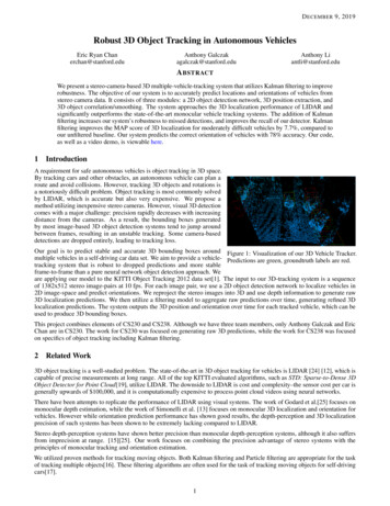
D ECEMBER 9, 2019Table 2: Mean Average Precision comparison of our unfiltered, Kalman filtered, and Particle filtered results against state-of-the-artMonocular and LIDAR vehicle-detection systems.Unfiltered Kalman Particle Mono[13] LIDAR[19]EasyMedHard0.7990.37370.1198Figure 5: PR curve for 2D tracking vs.3D e 6: PR curve for each distancethreshold, using Kalman filtering.Figure 8: Confusion matrix for orientation gure 7: PR curve for filteringmethod comparison.Figure 9: PR curve for each KITTI difficulty.Localization PerformanceFigure 9 and Table 2 compare the performance of our 3D tracking system at different difficulties. Our system performs verywell on “Easy” detections–vehicles that are fully visible and relatively close to the camera. Our system has lower performanceon vehicles that are far away and partially or significantly occluded, but still performs adequately. These results indicate thatas expected, localization precision decreases with increasing distance to the cameras. Additionally, localization precision isworsened by large occlusions.Figure 6 gives average precision curves for our system at different distance thresholds. Our system is able to localize the majorityof vehicles to within 1.5 m of their real-world positions. It is able to localize nearly all vehicles to within 3 m of their real-worldpositions. Our system, especially at long ranges, is not perfectly precise, and will not give millimeter-perfect localization.However, we contend that the precision is adequate for most autonomous vehicle tasks.5.2Orientation Prediction PerformanceThe confusion matrix given in figure 8 compares our predicted orientations to groundtruth orientations. Our system correctlypredicts the orientation of cars 76.8% of the time. The most common prediction errors are between adjacent angles. For example,the network is more likely to predict a front-facing car to be diagonal than it is to be completely sideways.Because many training images are taken from highway driving, the KITTI dataset is heavily biased towards front-facing cars.There are few training images captured at intersections, so the performance of “side” predictions is comparatively low. Webelieve that additional training examples with more varied orientations would improve our network’s orientation predictionperformance.4
D ECEMBER 9, 20195.3Filtering performanceWe evaluated the 3D localization performance of three different filtering models: an unfiltered baseline model, a particle filteredmodel, and a Kalman filtered model. The precision-recall curves for 3D localization with particle filtering and Kalman filteringare compared to unfiltered results in Figure 7. MAP values for the three filtering methods are given in Table 2.Kalman filtering improved baseline 3D localization performance for all three difficulties. However, the greatest improvementscame in localizing medium and hard vehicles, where Kalman filtering improved MAP by 7.7% and 5.9% respectively. Filteringprovides two benefits: robustness to dropped predictions and smoothing of sensor noise. The raw prediction system sometimesfails to detect vehicles that are difficult to detect, “dropping” predictions. Our filtering solution provides robustness to droppedpredictions by propagating tracked vehicles. When our object detector fails to predict a vehicle for 1-2 frames, the filter continuestracking through the brief loss of detection, updating the position of our estimate using our constant-velocity assumption.Additionally, by aggregating multiple noisy samples over time, Kalman filtering allows us to extract a better estimate of a trackedvehicle’s true position, making the system more resistant to sensor imprecision.66.1DiscussionComparison to LIDARTable 2 compares our localization performance to a state-of-the-art LIDAR vehicle-detection system, STD: Sparse-to-Dense 3DObject Detector for Point Cloud[19]. As expected, LIDAR outperforms our model at all difficulties. However, Figure 6 showsa compelling result when we relax the constraints on how precise the detections need to be. The performance of our modelincreases dramatically when we relax the detection distance threshold to 3 m. The takeaway is that although our system lacks thefine-grained precision of LIDAR, it can still adequately track most vehicles.Our system achieves comparable precision to LIDAR for vehicles that are “Easy” to detect, but performs significantly worse formore difficult vehicles. Many of these difficult to detect vehicles are cars that are smaller than 40 pixels in image-space height,i.e. cars that are far away from the cameras. Part of our tracking difficulty likely comes from the inherent imprecision of stereodepth perception at longer ranges, where LIDAR possesses a significant resolution advantage. However, precise tracking atlong range is often unimportant to autonomous vehicle tasks, where nearby objects pose the greatest collision risk. Because oursystem is comparable to LIDAR at close range, we believe it offers a compelling alternative to LIDAR.6.2Comparison to Monocular 3D object trackingTable 2 compares our localization performance to a state-of-the-art Monocular 3D vehicle detection system, DisentanglingMonocular 3D Object Detection by Simonelli, et al. [13]. Our system significantly outperforms the monocular object detector,achieving a 450% MAP improvement for “Easy” detections and a 270% improvement for “Medium” difficulty vehicles whileperforming comparably for “Hard” vehicles. Note that the monocular object detector MAP values are evaluated at a distancethreshold of 2 m compared to our less-forgiving default threshold of 1.5 m; the performance gap would likely increase further atthe same distance threshold.6.32D vs. 3D object trackingFigure 5 compares the accuracy of our 2D predictions to that of our 3D predictions. 2D detection performance is significantlygreater than 3D detection performance. This is partially due to the "dimensionality curse"–the much larger scale of the 3Dvolume makes 3D localization an inherently more difficult problem.However, the performance gap is also due to the limitations of our stereo ranging system. Our 3D detector performs much worseon vehicles that are significantly occluded. When objects are significantly occluded, our ranging method, which operates onthe principle of median filtering, sometimes returns the distance to the occluding object rather than the occluded vehicle. Wehypothesize that a more robust ranging algorithm could produce significant performance improvements for difficult vehicles. Forexample, if our model were to semantically segment the image, it could identify portions of the image that would produce themost accurate depth result, ignoring occluding objects.6.4Prediction AssociationWe examined several approaches for correlating raw 3D detections with tracked vehicles, known as “solving the data as
network did not generalize well and our performance was generally worse than with the pure RGB approach. 4.2 3D Position Extraction Figure 4: Diagram illustrating steps in our 3D Vehicle-Tracking System. After localizing vehicles in 2D image space, we used stereo correspon-dence algorithms to estimate the