WIXLIB

Single-Sample andTwo-Sample t Tests6IntroductionThe simple t test has a long and venerable history in psychologicalresearch. Whenever researchers want to answer simple questionsabout one or two means for normally distributed variables (e.g., neuroticism, daily caloric intake, height, rainfall), a t test will often provide theanswer to such questions. In the simplest possible case, a researcher mightwant to determine whether a single mean is different from some knownstandard (e.g., an established population mean). For example, a researcherinterested in the academic qualifications of Dartmouth students mightwant to see if the SAT scores of Dartmouth students are higher than thenational average. If the researcher had access to a small but representativesample of Dartmouth students, she might obtain their SAT scores (let’s saythe mean was 1190) and conduct a statistical test to see if this mean issignificantly higher than the national average (it fluctuates around 1000;let’s say it’s 1023). As you may recall, the formula for the single-samplet test ist M µ,SMwhere M is the sample mean about which you would like to draw an inference (in this case, 1190), m is the hypothetical population mean (1023)against which you would like to compare your observed sample mean, andSM is the standard error of the mean. The standard error of the mean isclosely related to the estimate of the population standard deviation, but italso takes the size of your sample into consideration. More specifically, it’sSM Sx.N161

162INTERMEDIATE STATISTICSAs your sample size gets larger, your estimate of the standard error of themean gets smaller, and this is why single-sample t tests (like almost allother statistics) become more powerful (i.e., more likely to detect a trueeffect, if there is one) as sample size increases. As a concrete example, suppose that you only had access to a measly sample of four Dartmouth students, whose mean SAT score was 1190 (as noted previously). Furthermore,suppose you didn’t know that the population standard deviation for theSAT is 100 points—and thus you had to estimate the standard error of themean for the SAT by first estimating the population standard deviation forthe SAT (based on your sample of four randomly sampled Dartmouthstudents). Let’s say this estimate of the standard deviation turned out to be114 points. According to the formula for a single-sample t test, the t valuecorresponding to your mean of 1190 would be1190 1023,57which turns out to be 167/57, which is 2.93.The critical value of t with 3 df (a .05) is 3.18. Thus, based on thissingle-sample t test, we would not be able to conclude that the mean SATscore of Dartmouth students is significantly greater than the national average. However, if we obtained the same mean and the same estimate of thestandard deviation in a random sample of nine rather than four Dartmouthstudents, our new estimate for the standard error of the mean would be 38rather than 57 (you should be able to confirm why this is so with some veryquick calculations). The t value corresponding to this new test would be4.39, and the new critical value for t with 8 df is 2.31. Even if we set alpha atthe more stringent .01 level, the new critical value would be 3.36, and we’dbe able to conclude (quite correctly, of course) that Dartmouth studentshave above-average SAT scores. Finally, if we had a random sample of 100Dartmouth students at our disposal, and we observed the same values forthe mean and the standard deviation, the resulting value for a single-samplet test would be 14.65, a very large value indeed. We would have virtually nodoubt that Dartmouth students have above-average SAT scores.So the single-sample t test can answer some important questions whenyou have sampled a single mean. To be blunt, however, many questions ofthis type are pretty darn boring. Most interesting psychological questionsusually have to do with at least two sample means. In an experiment, thesetwo means might be an experimental group and a control group. In a survey study of gender differences, these two means might represent men’sand women’s problem-solving strategies or the strength of their preferences for the initials in their first names (by the way, women like their firstinitials even more than men do).Back in the good old days, a lot of psychological studies could be analyzed using a two-sample t test. That is, many studies focused on (a) a single

Chapter 6  Single-Sample and Two-Sample t Tests163independent variable and (b) a normally distributed, or quasi-normallydistributed, dependent variable. For example, a classic social psychologicalstudy by Hastorf and Cantril (1954) examined people’s reactions to a bitterly contested football game between Princeton and Dartmouth (back inthe days when these schools had highly respectable teams). The only independent variable in this classic study was whether the observers of the gamewere enrolled at Princeton or at Dartmouth. One of the main dependentvariables was students’ estimates of the total number of penalties Dartmouthcommitted during the game (the researchers also looked at estimates of thenumber of penalties Princeton committed, but we’ll focus on Dartmouthbecause these results were the most dramatic). Because you live in the eraof controversial murder trials, controversial NFL playoff games, and controversial presidential election counts, you probably won’t be too surprisedto learn that the Princeton students and Dartmouth students strongly disagreed about just how many penalties Dartmouth had committed—evenafter reviewing a film of the game. However, back in the 1950s, many peoplesubscribed to the view that there is a single reality out there that most honest, self-respecting people can easily detect. How hard is it, really, to keeptrack of blatant infractions on film during a football game? Hastorf andCantril documented that it could be quite hard indeed. Whereas the averageDartmouth student estimated that Dartmouth committed 4.3 infractionsduring a sample film clip, the average Princeton student put the total number of infractions at 9.8 after observing the same film clip. A two-samplet test confirmed that these different estimates were, in fact, different. Thist test thus indicated that, even after viewing the same segments of gamefilm, the student bodies of Princeton and Dartmouth strongly disagreedabout the number of infractions committed by Dartmouth.In this chapter, we are going to examine the t test and explore some ofits most common uses. We begin by examining a simple data set thatrequires us to conduct a one-sample t test. Because the single-sample t testis conceptually similar to certain kinds of χ2 tests, we will compare andcontrast the single-sample t test with a χ2 analysis based on the samesimple study. Next, you will examine some simulated data from a classicfield experiment using both an independent samples t test and a twogroups χ2 test. After warming up on these two activities, you will use t teststo examine three other data sets, including a name-letter liking study, anarchival study of heat and violence, and a blind cola taste test. Let’s beginwith the data involving inferences about a single score or mean.Bending the Rules About HappinessA cognitive psychologist was interested in the function rule that relates happiness to the objective favorability of life outcomes. Because of the preliminary nature of her research, she wanted to begin by testing her most

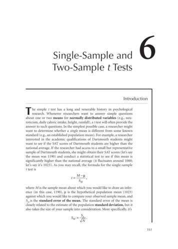
164INTERMEDIATE STATISTICSbasic assumption about the perception of happiness. In particular, theresearcher assumed that as the objective favorability of a positive outcomeincreases in a linear fashion, people’s subjective, psychological responses tothe outcome will not increase in a linear fashion. Instead, she felt that subjective happiness will follow what might be termed a law of diminishingreturns. As events become objectively more favorable in a linear fashion,people will only experience them as more favorable in a diminishing, curvilinear fashion. For example, based on past research, this researcher knewthat if we wish to double the perceived intensity of a light presented in anotherwise dark room, we will have to increase its physical (i.e., objective)intensity by a factor of about 8. To be perceived as twice as bright as LightA, Light B must emit about eight times the amount of light energy as LightA (e.g., see Billock & Tsou, 2011; Stevens, 1961). Does this simple rule ofdiminishing returns apply to emotional judgments such as happiness? As afirst test of this idea, the researcher asked people to think about how happythey would be if they were given 10 dollars. She then asked them to reportexactly how much money it would take to make them exactly twice thishappy (see Thaler, 1985). Her reasoning was simple. If the law of diminishing returns applies to happiness, it will take more than 20 to make theaverage person twice as happy as he or she would be if he or she were toreceive 10. Image 1 depicts an SPSS data screen containing data from 20hypothetical participants who took part in this simple study. You shouldconvert the screen capture in Image 1 to an SPSS data file of your own.21After making sure the scores in your data file look exactly like those inImage 1, click “Analyze” and then go to “Compare Means” and “OneSample T-Test. . . .” Clicking on this analysis button will open a dialog boxlike the one you see in Image 2. Send your only variable (“howmuch”) to

Chapter 6  Single-Sample and Two-Sample t Tests165the Test Variable(s) list, and enter 20 as your Test Value (circled in Image 2).Now click the “Paste” button to send this one-sample t test command to anewly created syntax file. Your syntax file (especially the text) should lookvery much like the one you see in Image 3.43Running this one-sample t test command (by clicking the “Run” button)should produce an output file that looks a lot like the one you see in Image4. We will leave it up to you to decide exactly what each piece of information in this output file tells you about the results of the researcher’s study.QUESTION 6.1a. Summarize the results of this study as if you had conductedthe study yourself. Make sure to include everything you would want readers toknow about your results. First, briefly explain why you set 20 (vs. 0, 100, etc.)as your comparison standard. Defend this choice against the (incorrect) criticism that one-sample means are supposed to be compared with some kind ofpopulation value (e.g., population SAT scores). Second, be sure to describeyour findings relative to this comparison standard (e.g., “Dartmouth studentsexceeded the population mean on the SAT by more than 30%.”). In otherwords, what, exactly, did you find? Third, was this finding statistically significant? Report your observed t value the way you would report it in a researchpaper. In case you are not familiar with the format for reporting the results ofa one-sample t test, some examples appear in Appendix 6.1.QUESTION 6.1b. Just to keep you on your toes, work from the information given in your printout and check to be sure that SPSS (a) correctlyconverted the standard deviation to the standard error of the mean and(b) correctly calculated the value of the t test itself. Make sure to show yourwork for these hand calculations. (Do not start from scratch. Instead,merely use the values for the sample mean and standard deviation that youare given in your SPSS output file.)