Transcription
TensorFlow to Cloud FPGAs: Tradeoffs forAccelerating Deep Neural NetworksStefan Hadjis and Kunle OlukotunDepartment of Computer Science, Stanford University, Stanford, CA, USAEmail: shadjis@stanford.eduAbstract—We present the first open-source TensorFlow toFPGA tool capable of running state-of-the-art DNNs. RunningTensorFlow on the Amazon cloud FPGA instances, we providecompetitive performance and higher accuracy compared to aproprietary tool, thus providing a public framework for research exploration in the DNN inference space. We also detailthe optimizations needed to map modern DNN frameworks toFPGAs, provide novel analysis of design tradeoffs for FPGA DNNaccelerators and present experiments across a range of DNNs.I. I NTRODUCTIONDeep Neural Networks (DNNs) provide state-of-the-art results in many industries [1]. Many companies have turned tocustom hardware accelerators for DNN processing to achieveimproved throughput, latency and power compared to GPUsand CPUs [2], [3]. In particular, programmable acceleratorslike FPGAs are useful because computations vary acrossDNNs and algorithms often change. However, designing programmable accelerators requires a long development process,and DNN accelerators pose unique challenges due to the sizeof their design space and the complexity of modern DNNs.The first challenge is that designing an accelerator fora given DNN requires a number of choices, ranging fromaccelerator architecture to memory management. In addition,design decisions change based on properties of the DNN, suchas layer types and data structure sizes. Exploring architecturesto optimize for these considerations involves a large designspace and complex implementation process.In addition, due to their complexity, DNN applicationsare almost always developed using high-level frameworks.TensorFlow [4] from Google is the most popular. As of 2019it is the top machine learning framework on GitHub.com. Thisleads to a second challenge, because efficiently running a DNNexpressed at a high-level on a low-level programmable hardware target requires optimization at many levels of abstraction.To solve these problems, we develop an end-to-endtoolchain to go from high-level DNN models to low-levelhardware. The input is a TensorFlow model and the output isan optimized FPGA design. Formats from other frameworksalso can be swapped in. Our toolchain supports FPGAs frommultiple vendors, but here we focus on the recently announced,publicly available Amazon cloud FPGAs [5], [6].This solves both problems above: it allows easily experimenting with architectures and algorithms to explore largedesign spaces, and it performs the required optimizations ateach level of the stack so DNNs expressed in a high-levelframework can be efficiently deployed to hardware. We hopethat our toolchain, which allows DNNs to be expressed inmodern formats and targets public hardware, can help theFPGA community research DNN accelerators. The code islinked below1 . We make the following contributions:1) We study the optimizations needed to start from a modernDNN framework and efficiently map to FPGAs. This includesDNN optimizations overlooked in the FPGA literature andrecommendations to improve existing tools.2) We provide novel experimental analysis of tradeoffs inthe FPGA DNN accelerator design space, providing insightsinto generating efficient DNN FPGA hardware.3) We provide an open, end-to-end toolchain to accelerateTensorFlow DNNs on FPGAs. It is capable of running onpublicly-available cloud FPGAs and compiles DNNs achievingstate-of-the-art accuracy (the first open-source TensorFlow toFPGA compiler to do either of these). It also automaticallyperforms state-of-the-art optimizations from the literature,allowing it to be used as a research tool for design exploration.Next we describe the space when designing an FPGAaccelerator for a given DNN, and how design choices areimpacted by various factors.II. T RADEOFF S PACE FOR DNN ACCELERATORSGiven a DNN to accelerate, this section discusses accelerator design choices and factors influencing them. DNNs arecomposed of layers arranged in a dataflow graph. The numberof layers can range from a dozen to hundreds. Example layersinclude convolution and pooling [1]. Each layer transforms aninput tensor (multi-dimensional data array) to an output tensor.These tensors of data are also called “activations”. Some layersalso contain model parameters (sometimes called weights orkernels) which are read-only, e.g. convolution filters.For clarity we partition the design space into three components: architecture, memory management and accuracy tradeoffs. In this work we focus on the first two. Accuracy tradeoffsinclude approximations like lowering precision or changingthe DNN model, which may give speedups but also impactcorrectness. We discuss precision in Section 5, but otherwisethis work focuses on accelerating a DNN as-given.Fig. 1 describes the design space related to architectureand memory management, as well as factors which impactdesign choices. Architecture design determines the coarsegrained computations the architecture must support (e.g. whichDNN layers) as well as core computational units of the accelerator’s processing elements, for instance whether convolutions1 https://github.com/stanford-ppl/spatial-multiverse
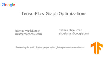
Accelerator ArchitectureExamples of Design ChoicesFactors Influencing Choices Granularity of operations to support Algorithm choice (e.g. convolution asGEMM vs. sliding window) General architecture for multiple layertypes vs. per-layer specialization Types of layers in DNN (affectsrequired operations in hardware) Amount of variation across layeroperations (determines benefitsof specialized hardware)Memory ManagementExamples of Design ChoicesFactors Influencing Choices Tensor storage format (major dimension) Locality properties of layer Parallelism in the memory system (e.g.computationssimultaneous DRAM accesses) If layers are compute-bound On- vs. off-chip storage of data structures Model/data size (if it fits on-chip)Fig. 1. An overview of common choices when designing DNN acceleratorsas well as factors influencing these choices.should be performed as dot products or a sliding window(stencil). Another decision is whether different types of DNNlayers should be implemented by specialized processors orwhether multiple layer types should share a single, moregeneral processor. Whereas an ASIC DNN accelerator mustsupport a variety of DNNs [7], the reconfigurability of FPGAsallows accelerator designs to be specialized for a specificDNN. Therefore the number of DNN layers, the types ofcomputations they perform and the degree of layer variabilityimpact architecture design choices.Memory management choices include where data structuresshould be stored in memory, the formatting of these datastructures in memory and the amount of parallelism in thememory system to eliminate memory bottlenecks. DifferentDNN layers have different locality properties and arithmeticintensity [2],therefore the types of DNN layers as well as thesizes of their data structures also impact design choices.The space is large, and our next step is to design an endto-end toolchain which can explore this design space startingfrom a high level of abstraction.III. OVERVIEW OF C OMPILEROur compiler allows DNNs developed in high-level frameworks to be efficiently deployed to FPGA hardware, andperforms the required optimizations at each level of the stack.It contains three Optimization Levels, shown in Fig. 2.A. Level 1: DNN-Specific OptimizationsLevel 1 processes the DNN graph to perform optimizationsthat will later help hardware generation. DNN frameworksrepresent a DNN as a data-flow graph (DFG), where nodes areoperations (e.g. Convolution) and edges are data tensors passedbetween them. TensorFlow and other modern frameworks (e.g.ONNX) contain utility tools to perform graph optimizations,e.g. constant folding. However, it is often not obvious tothe DNN framework that certain optimizations apply and theburden is placed on the user to perform graph processing.Table I shows an example of how various optimizationssimplify the TensorFlow DFG for the popular ResNet-50 [8], astate-of-the-art CNN. Each row corresponds to an optimizationrun by our script. The first row is the downloaded model afterusing TensorFlow’s API to create the inference graph, whichfreezes variables to constants and removes training nodes.TABLE IO PTIMIZATIONS ON THE R ES N ET-50 T ENSOR F LOW GRAPHDescription# DFG Nodes Needs RSqrt Needs ScaleFreeze for Inference460YesYesFold Constants354NoYesFold BatchNorms301NoNoNext we run optimization passes. These are not automatically performed by TensorFlow (or ONNX) when freezingfor inference so they need to be run separately. In the ResNetexample, two optimizations help for custom hardware. Bothare related to constant folding and regard the layer patternof Convolution followed by Batch Normalization (BN), whichoccurs 53 . When converting variables to constants, foldingopportunities arise for operations which differ in the forwardpass of training vs. inference, such as Dropout or BN.The first optimization is noted by prior FPGA work [9],[10]. It eliminates reciprocal square roots and other operationson tensors of constants: BN computes statistics on the data butduring inference these are constants and can fold into a linearfunction. The result is shown in the second row of Table I.The second optimization however is overlooked by priorFPGA work. It eliminates the tensor scaling operation ofBN by folding the constant scaling factors of BN into theConvolution before the BN. This updates the already-trainedConvolution weights to incorporate the BN scaling factors,and replaces BN with a simpler bias addition which requiresno multiplication. The third row shows this final result. PriorFPGA work computes both the scaling and addition components of BN, e.g. recent work still remarks how BN needs“multipliers that are expensive” [11]. We therefore suggestFPGA tools move to modern frameworks to get these benefits.Finally, optimization utilities can fail for DNNs with controlpaths, e.g. when selecting operations that differ from trainingto inference. In such cases our scripts also perform a traversalto first fold constant branch inputs through control nodes(Switch, Merge) and eliminate unused subgraphs.B. Level 2: Optimizations for DNN Hardware AcceleratorsLevel 2 contains the majority of the optimization and isthe focus of Section 4. It converts the optimized DNN graphfrom Level 1 into a Hardware IR describing the circuit. Thisspecifies the exact architecture layout of the DNN on-chip.C. Level 3: DNN-agnostic, Target-specific OptimizationsLevel 3 compiles the Hardware IR into synthesizableVerilog and makes optimizations for the target FPGA. Ourcompiler uses the open-source High-Level Design languageSpatial [12] as the Hardware IR. It provides hardware-specificabstractions, i.e. it is more like a high-level HDL than ahigh-level synthesis (HLS) tool. We chose Spatial becausethese abstractions allow fast prototyping without sacrificingknowledge of the synthesized circuit, e.g. by allowing usersto explicitly control memory hierarchy (DRAM, SRAM, FFs).While a strength of HLS is that it allows software engineersto make fast progress, for our toolchain the user’s entry pointis already TensorFlow. We therefore opted for an IR whichgives more control over the underlying circuit.
DNN Graph inModern Framework(or otherframeworks)Input DNNDNN Graph optimizedfor inferenceDNN GraphOptimizationRun scripts thatuse TensorFlowAPI and utilitiesDesign specified inHardware IR (Spatial)Specify DNN Hardware ArchitectureAssign operations toAlgorithmFuse layershardware (determineselectioninto coarserlevel of specialization,for fusedoperationsselect parallelizations)operationsVerilog Design andC Host izationsGenerate HDLusing area /timing modelsOptimization Level 2Optimization Level 3Optimization Level 1Fig. 2. A detailed view of the compiler flow, showing optimizations at each level of the stack.At the same time, because the goal is to explore algorithmsand architectures, describing hardware at a higher level thanVerilog is helpful. Spatial facilitates this by performing optimizations like pipeline scheduling to exploit parallelism andmemory banking to reduce on-chip memory usage. It alsoperforms automated tuning of parameters such as operatorlatencies based on FPGA-specific timing models. Finally, itis open-source and supports FPGAs from multiple vendors,including being one of few tools to support the Amazon cloudFPGAs. The output of Spatial is a Verilog design for the FPGAand a C program which runs the design from the host CPU.Our DNNs were larger than previous Spatial applicationshowever, so modifications were needed to improve performance. First, we modified Spatial’s interface between theapplication and the Amazon-provided shell to delete unusedIPs, reducing LUT and BRAM utilization by 8% and 19%of the total available. Second, we wrote an analysis passto assign SRAM data structures with size 1024 wordsto UltraRAMs (URAMs), which are deeper block RAMs onXilinx UltraScale FPGAs that were unused by Spatial. Third,a challenge in designing CNN hardware is that irregular sizeparameters are ubiquitous (e.g. 3 3 convolution kernels, 7 7feature maps). These odd numbers lead to complex accesspatterns when performing sliding window computations whichSpatial was not optimized for. This resulted in large LUToverheads after SRAM banking because banking schemesusing non-powers of 2 were selected, which used expensiveinteger division and modulus to calculate addressing. OurDNNs drove improvements to Spatial’s banking, including (1)banking support for more general access patterns to eliminateunnecessary crossbars and address calculation, and (2) modifications to Spatial’s banking algorithm to automatically bankmulti-dimensional SRAMs with parallel accesses. These ledto a more than 2 reduction in LUTs for some applicationsand are now part of Spatial’s official repository.In Summary, compiler Levels 1 and 3 leverage and improve third-party, open-source tools to improve DNN hardwareperformance. Level 2 is entirely within our framework andconverts the optimized TensorFlow DFG to a program in theSpatial Language. We now describe Level 2 in more detail.IV. DNN-H ARDWARE O PTIMIZATIONS AND D ESIGNE XPLORATIONOptimization Level 2 converts the DNN DFG to HardwareIR. It involves three steps, shown in Fig. 2 (center). We nowdescribes these, with emphasis on exploring design tradeoffs.As a running example we consider the ResNet-50 CNN [8].Compute BoundWeightMem. BoundWeight(or otherFPGAs)DeployMem. Bound Mem. BoundInputPoolReLUConvBNormDataFig. 3. An example of a frequently occurring layer pattern in CNNs. It ismore efficient to fuse this into a single coarse-grained operation.LayerCountConv 7x7, Stride 21Conv 1x1, Stride 130Conv 3x3, Stride 116Conv 1x1, Stride 26Pool (Avg, Max)2Batch Norm53ReLU49Tensor Add16Fully-Connected1OperationFused Conv 7x7, Stride 2Fused Conv 1x1, Stride 1Fused Conv 3x3, Stride 1Fused Conv 1x1, Stride 2Tensor AddFully-ConnectedCount130166161Fig. 4. ResNet-50 layers (left) and the coarse-grained operations they aregrouped into after fusion (right).A. Identify coarse-grained operations (fusion)The first step selects the granularity of hardware operationsto compose the DNN. Often, DNN layers occur in repeatingpatterns. Fig. 3 shows a common example in CNNs: Convolution/BN/ReLU/Pool. This pattern appears twice in ResNet-50and the smaller pattern of Conv/BN/ReLU appears 53 .Fusion is a state-of-the-art technique for DNN acceleratorswhich minimizes DRAM bandwidth [13], [14]. As Fig. 3shows, all but the Convolutional layer contain little computation and are bound by the time to access DRAM. It is thereforebeneficial to fuse these layers into a single, more coarsegrained operation. This loads the data from DRAM once,performs all the layers in the operation without separatelymaterializing the output of each, then stores the result afteronly the final layer. In this way, fused layers communicateusing SRAM and registers to minimize DRAM bandwidth.Our compiler performs fusion by matching for commonpatterns within the graph. Once a layer pattern is matched,the layers are replaced with the fused operation. Fig. 4 showshow the operations change in ResNet-50 after fusion. Withthese fusions applied, the arithmetic intensity of ResNet-50inference, measured in Ops/byte (as in the Roofline modelsused by [2], [15]), improves by 2.55x.B. Algorithm-Level TransformationsThe next step considers algorithm-level transformations onfused operations to identify efficient hardware for each. Revisiting the example from Fig. 4, note there are two major types ofoperations: 1x1 and 3x3 convolutions (Tensor Add is computationally inexpensive and also can be fused into other layers).“1x1” and “3x3” refer to the filter size (rows columns). Othermodern DNNs also primarily use smaller convolutions, andthese sizes (1x1, 3x3) have become most common.
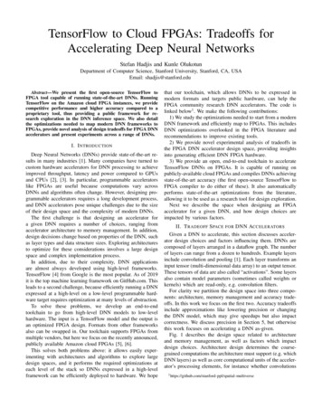
3D Tensor:3a 3b 3c3d 2a 2b 2c3g 2d 1a 1b 1c2g 1d 1e 1f1g 1h 1iRow-Major Format:1a 1b 1c 1d 1e 1f 1g 1h 1i 2a 2b 2c 2d Feature Map 1Channel-Major Format:1a 2a 3a 1b 2b 3b 1c 2c 3c 1d 2d 3d 1e Pixel A for all channelsFig. 5. Two popular storage formats for 3D data tensors in CNNs.1x1 convolutions have lower arithmetic intensity and somelocality in the 2D spatial dimension (rows columns). 3x3convolutions have higher arithmetic intensity and more localityin the 2D spatial dimension. Recall that convolutions in CNNsoperate on 3D tensors of data, which consist of a series of 2D“channels” or “feature maps”. The convolution involves slidinga series of filters across the rows/columns of each channel,creating 2D locality. Moreover, at each step of the slidingwindow, a 2D dot product (e.g. 3x3) is performed, furtherincreasing locality. The convolved results of each channel arethen added together to produce a single channel of output(output feature map). This sum now creates locality in thechannel dimension. Finally, the process is repeated for multiplesets of filters to produce multiple output channels.While the loops comprising this algorithm have been studiedfor DNN accelerators [16], [17], prior work often overlooksthe storage format of these 3D tensors. Fig. 5 shows thetwo popular data storage formats in DRAM used by DNNframeworks and accelerators: row-major and channel-major.Each format is better suited to a different algorithm forconvolution. Row-major (rows contiguous in DRAM) is bettersuited to convolution as sliding window, due to locality in therows/columns. Here the inner loops implement the 2D stencilsliding across the rows/columns, and then the outer loopssum each 2D result. Sliding window was used by [10], [14].Channel-major (channels contiguous in DRAM) is also useful,due to locality in the channels (convolution results from eachchannel are summed). In this case the outer loops implementthe 2D sliding window, while the inner loop performs a 1Ddot product along each activation and kernel channel [17].Fig. 6 shows the architecture for row-major format, whichuses sliding window convolution. Each PE loads input featuremaps from DRAM and performs convolution with a blockof kernels. The core computation (dot product) is each 2Dwindow reduction. The partial output feature maps from eachPE are then summed across channels to produce a block ofoutput feature maps. The architecture for channel-major is verysimilar, except that the dot products are 1D, and performedalong the channels of the kernels and activations. As a resultthe accumulation across channels is performed within each PEas part of the dot product rather than in the outer-loop.Fig. 7 shows experiments with the different data formats forboth major operation types in ResNet-50: 1 1 (left) and 3 3(right) convolution. The performance requirement is set to 1msfor 1 1 and 2ms for 3 3, and since tensor dimensions changealong the depth of a DNN, designs must meet this latency forsizes ranging from (rows, columns, in channels, out channels) (56, 56, 64, 64) to (7, 7, 512, 512), which is common forDNNs. For each layer type, we compare the two data formatsLoadiFMApActivations (DRAM)iFMapsPEPEPEActivation BufferBroadcastPEDotProdChannel AccumulatorFused OperationsDotProdKernel BufferK2K3K4DotProdDotProdoFMap 1oFMap 4oFMap 2 oFMap 3(b) Processing EngineActivation Buffer(c) Dot Product Engines- Special-cased for k- When k 1 (1x1 conv),no reduction neededK1Partial SumsStore block of oFMaps(a) Architecture OverviewLoad blockof kernelsk0Activation Bufferk00 Dot Product Engine,1x1 special-casek01 . . . k2 . . . Dot Product Engine, for a k x kFig. 6. Architecture overview for tensors stored in row-major format.and their associated algorithm.For 1x1 convolution, both formats use similar resources asthere is locality both in the channels as well as rows/columns.For 3x3 convolution, now row-major benefits from additional locality in the rows and columns. With channelmajor, overlapping regions of the sliding window need tobe loaded multiple times from DRAM, increasing bandwidthrequirements. To meet the same performance, larger bufferswere needed for channel-major to store more kernels on-chipat once. This reduced the number of times the data is re-loadedfrom DRAM, but increased logic and memory utilization.Overall, due to locality, row-major is more efficient for largerconvolution sizes. Choosing this incorrectly results in a 2 increase in BRAM/URAM end-to-end for ResNet.There is some prior work which also finds the data formatsbest-suited to their architecture [9], [18], but we are the firstto quantify the costs of choosing incorrectly by comparingformats experimentally. Also, [9] focused on small DNNswith small input images (32 32). Such smaller data structuresmay not reflect real-world applications and could change thelocality analysis. Our work compares data structure formatsexperimentally for larger inputs used by modern DNNs, andwe are the first to measure how format impacts different algorithms and convolution sizes based on locality, in particularfor convolutions of the sizes used by ResNet-like DNNs.Based on these experiments, our compiler selects defaultsettings for data format and algorithm. While we described onealgorithm tradeoff related to memory format, our toolchain canbe used to explore others, e.g. FFT or Winograd convolutions.We also observed while optimizing for each format that sometimes algorithms ran into memory bottlenecks, yet were not atthe intrinsic DRAM bandwidth. This was because bottleneckswere in memory access logic, e.g. generating addresses anddequeuing from FIFOs. The customizability of FPGAs allowedus to solve this by introducing parallelism into the memorysystem, e.g. creating parallel channels to the DRAM controllerand allowing PEs to issue simultaneous DRAM commandsto hide memory access latencies. This eliminated memorybottlenecks and made execution compute-bound, allowing usto use a static model for runtime and resources to selectparallelizations. We describe this in the following subsection.
% Utilization1008060402001x1 row-major1x1 channel-major22 21 23 15 19283x3 row-major3x3 channel-major82 87 8720 203245Conv 7x7 Stride 2541628LUT BRAM URAM DSPBRAM URAM DSPResourceResourceFig. 7. Resource Utilization vs. Data Format for 1x1 (left) and 3x3 (right)convolutional layersLUTC. Assign Operations to HardwareThe final step assigns operations to hardware and schedulestheir execution. This involves determining the right degree ofspecialized hardware per DNN operation. We build on thestrategy from [17], which takes advantage of the FPGA’s flexibility to instantiate a specialized processor for each operationtype. They show that specializing portions of the FPGA fordifferent convolutions increases performance more than 2 over a single, more general architecture shared by all layers,and that this gap grows for larger FPGAs (like on the Amazoncloud). A limitation of [17] however was that the approachwas not detailed for the deeper, state-of-the-art networks likeResNet. Moreover, it considered only convolutional layerssimulated in isolation and not entire DNNs running end-to-endin hardware. We therefore extend their analysis and explore towhat degree this strategy applies to entire, modern DNNs.Returning again to the ResNet-50 example of Fig. 4, notethat 6/36 of the 1x1 convolutions have stride 2. The hardwareof Fig. 6 is the same regardless of stride as it just skips computations in the sliding window, therefore all 1x1 operationsmap to a single processor with no overhead. Stride was notdiscussed by [17], and so we here report that different stridescan map to the same processor without penalty.We also mapped the 1x1 and 3x3 convolutions to a singleprocessor, but there was no net area reduction from mergingthese two. While merging did instantiate one less processor,it added extra overhead due to the differences in control logic(Fig. 6c) needed when performing the window reduction for3x3 and 1x1. Separate processors also helped routability acrossstacked dies of the device. This extends the finding of [17] thatkernel specialization is still beneficial in modern DNNs.Our compiler therefore distinguishes operations by theirfused layer types, treating convolutions of different kernelsizes as separate types. It then instantiate one processor peroperation type, each like Fig. 6 and specialized to its operation,and creates an FSM which executes the fused operationssequentially on their associated processor, writing intermediatedata to DRAM. The architecture for the ResNet example isshown in Fig. 8. Our compiler statically calculates the numberof total multiply-accumulates (MACs) contributed by eachoperation type, and allocates DSP resources proportional tothat (rounded to a power of 2). We show these details nextto each processor, and for reference include the percentage ofruntime for a single inference. The totals, described further insection 5, are the total MACs in ResNet-50, total DSPs usedby the design and total inference time. The result is that theruntime is balanced between two processors, 1x1 and 3x3, asDRAMSRAMBuffers(BRAM,URAM)%Ops3%Conv 1x1, Stride 1,2(special-case1x1 reduction)Conv 3x3, Stride 1(3x3 slidingwindow)Tensor AddFully Connected%DSPs %Runtime8%7%49%43%48%48%48%40% 1% 1%0% 1%3%2%Fig. 8. Overview of architecture for ResNet example.expected from Fig. 4. These can be used simultaneously byprocessing two inputs at once, as described in [17].This section described the optimizations needed to transform a DNN DFG into a synthesizable circuit. We performedexperimental analysis of the design choices summarized inFig. 1, including operation granularity (fusion), hardwarespecialization, algorithm transformations, data format, andmemory-level parallelism. Next, we measure the performanceof various DNNs mapped to hardware using this toolchain.V. E XPERIMENTSWe consider 4 benchmark TensorFlow DNNs from variousmultimedia applications in Table II. These were chosen toexercise a wide variation in the design space. ResNet-50is a complex graph containing a wide variety of layers asSection 4 showed. Djinn-ASR is a speech-to-text cloud serviceMLP [19] which contains fully-connected (FC) layers. UnlikeCNNs which process images, Djinn-ASR has small activationsbut a large model. TensorFlow CIFAR is the CNN used byTensorFlow’s tutorial for the CIFAR-10 dataset. LeNet is asmall CNN chosen because its weights and activations canfit entirely on-chip. These DNNs and datasets are commonlyevaluated in FPGA DNN papers [9], [14], [20].We ran these DNNs on the Amazon EC2 F1.2xlarge FPGAinstance, which contains a Xilinx UltraScale 16nm VU9PFPGA. The only other tool available which ran DNNs on theF1 was Xilinx’s ML-Suite (v1.3) [21]. As we will discuss, ourtoolchain can compile TensorFlow models that gave ML-Suiteerrors. First however, we compare speed performance.Table II compares single-input (batch-1) latency of theseDNNs. Microsoft argues batch-1 latency to be the most valuable metric for DNN data-center workloads [3]. We measureperformance of these DNNs for both our tool, which is anacademic research tool, and Xilinx’s ML-Suite, which is acommercial tool. ML-Suite is state-of-the-art, achieving sameor superior performance to GPUs [22] and running certainmemory-bound layers on the CPU using optimized BLAS [21].We match ML-Suite on all but ResNet, for which weare currently 5.7x slower. This is because of two majordifferences: (1) ML-Suite runs DSPs at 500 MHz, while wecurrently target the default 125 MHz for the F1, and (2) weuse 32-bit fixed point (10/22) and match the exact output ofTensorFlow, while ML-Suite uses 8-bit precision. Implementing these optimizations in our toolchain would result in 4xand 7.4x speedup respectively (discussed further below).Low precision causes problems however for ML-Suite. Theonly reasonable accuracy we could achieve from it was using
TABLE IIP ERFORMANCE AND R ESOURCE U TILIZATION OF VARIOUS T ENSOR F LOW DNN S RUNNING ON VU9P OF EC2 F1.2 XLARGE .DNNResNet-50Djinn-ASRTF CIFARLeNetTensorFlow FAR-101.06MMNIST430k#MAC3.9G25.4M19.5M2.29MXilinx ML-SuiteLatency (ms)38.110.71.201.01their pre-compiled ResNet-50 Caffe model (Caffe is an olderframework). When trying to compile TensorFlow through MLSuite, we followed the documentation and exhaustively triedsettings for both TensorFlow’s official ResNets as well as aXilinx-provided ResNet converted to TensorFlow from Caffe,and the highest Top-5 ImageNet validation accuracy we couldachieve was 12.1%, which indicates a bug in the TensorFlowcompilation. Though our tool uses higher precision, it matchesthe output of a CPU or GPU (93.2%). Overall, only our toolcould reasonably run the TensorFlow model on the F1. MLSuite c
simplify the TensorFlow DFG for the popular ResNet-50 [8], a state-of-the-art CNN. Each row corresponds to an optimization run by our script. The first row is the downloaded model after using TensorFlow’s API to create the inference graph, which f