Transcription
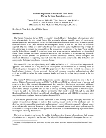
Seasonal Adjustment of CPS Labor Force SeriesDuring the Great Recession October 2013Thomas D. Evans and Richard B. Tiller, Bureau of Labor StatisticsBureau of Labor Statistics, Statistical Methods Staff,2 Massachusetts Ave. NE, Room 4985, Washington, DC 20212Key Words: Time Series; Level Shifts; RampsIntroductionThe Current Population Survey (CPS) is a monthly household survey that collects information on laborforce characteristics for the United States. The seasonally adjusted monthly levels of employment,unemployment and unemployment rate are key indicators of the health of the economy. Recent economicturbulence related to the Great Recession has raised public interest in how the CPS series are seasonallyadjusted. The most widely used approaches to seasonal adjustment apply weighted moving averages tothe original data to separate the seasonal from the nonseasonal components of the data. These weightsmay be derived from a model fit to each series or from a non-parametric method using pre-determinedfilters. These methods have been successful because of their flexibility in accommodating stochasticchanges in seasonal patterns. The presence of stochastic seasonality, however, creates conceptual andstatistical difficulties in separating seasonal from the nonseasonal components. The difficulties arecompounded during periods of rapid economic change.The national CPS data are adjusted using X-12-ARIMA (Findley, et al., 1998) which is a nonparametricapproach. This method has a long history of development and refinement and is currently used bystatistical agencies throughout the world. This paper reviews how well this method was designed tohandle changes in trend-cycle and seasonality during both economic expansions and contractions, whattools are available to adjust for major economic shocks, and how the method has performed in the lastrecession.The original X-11 filtering algorithm that performs seasonal adjustment remains at the core of the X-12process (Shiskin, Young, and Musgrave, 1967). The X-11 part of X-12 has a broad range of seasonal andtrend-cycle filters. The symmetric Henderson trend filter reproduces third-degree polynomials within thespan of the filter which can be as short as one to two years. Thus, the trend filter is flexible enough tofollow rapid changes in growth rates as well as quickly occurring turning points in the trend-cycle.Towards the end of the series less adaptive asymmetric filters must be used. Although the one-sidedHenderson filter is less flexible, it can still track a local linear trend and with ARIMA forecasting so moreadaptive filters are produced for the end points (Dagum 1983).A well-known problem with seasonal adjustment is that moving averages are highly vulnerable tosudden strong atypical changes or outliers. For example, sudden shocks to the trend-cycle can beabsorbed into the seasonal factor estimates and erroneously removed from the seasonally adjusted series.A second potential source of distortion is a break in the seasonal pattern which some analysts argue islikely to occur during recessions. Either type of shock may lead to distorted seasonally adjusted estimatesin later years following the recession.The best way to detect and correct for sudden disturbances is with prior information on their source,time of occurrence, magnitude, and duration. The original X-11 developers added an option for users to1 Disclaimer: Any opinions expressed in this paper are those of the authors and do not constitute policy of the Bureau of LaborStatistics.
supply adjustment factors to the original data to remove the effects of shocks prior to seasonal adjustment.Users, however, had to develop these prior adjustments outside of the software. This is hardly feasible todo when there are hundreds or thousands of series to seasonally adjust. With the addition of theRegARIMA modeling capabilities in X-12 (Findley, et al., 1998), it became standard practice to utilizethe automatic outlier detection routine prior to the seasonal adjustment step. RegARIMA also allowsusers to specify their own outlier models.Currently, there are 144 CPS national series that are directly seasonally adjusted. One hundred andthirty-nine of these series are released monthly and the others quarterly. Many more are indirectlyseasonally adjusted based on the directly-adjusted series. See Tiller and Evans (2013) for more details.The focus of this paper is on eight CPS series that make up the national unemployment rate:Employment (EM) ages 16-19 by genderEmployment ages 20 by genderUnemployment (UN) ages 16-19 by genderUnemployment ages 20 by genderThe eight series are directly seasonally adjusted and then used to derive the seasonally adjustedunemployment rate (UR). The official national seasonally adjusted unemployment rate is plotted overtime in Figure 1. The trend for the unemployment rate (not officially published) appears in Figure 2.Both series rise sharply in the 2008-2009 period. Commentary from Wall Street analysts and othermembers of the press suggested that the sharp rise (fall) in UN (EM) from the fourth quarter of 2008 tothe first quarter of 2009 was absorbed into the seasonal component and this caused seasonal adjustment tooverestimate recent economic growth in those quarters (a decline in UN or a rise in EM) andunderestimate in the second and third quarters.Testing for Trend-Cycle and Seasonal Breaks with RegARIMA ModelsTo investigate the claims of distortions to the seasonal adjustment process, we use RegARIMA modelsto test for the presence of recession effects due to trend-cycle and seasonal breaks. For seasonal breakswe also use a graphical analysis of X-11 seasonal-irregular (SI) sub-plots by month which will bedescribed in more detail below.The RegARIMA model may be represented as,yt Xt Ztwhere Xt is a vector of fixed regressors and Zt follows a seasonal ARIMA model. The parameters of theARIMA model implicitly determine the stochastic properties of seasonality as well as trend-cycle andother components of the series without having to specify specific models for these components. Thevariables of the regression part of the model provide the basis for testing for the presence of exogenouseffects, such as trend and seasonal breaks that we wish to estimate and remove from the series prior toseasonal adjustment to prevent distortions to the X-11 seasonal adjustment process.Trend breaks can be handled by modeling level shifts (LS), temporary changes (TC), and ramps whichare briefly described below and the form of the regression variables for testing for each effect are shownin Table 1. These variables are part of a large set of built-in regressors available in RegARIMA.
LS: A permanent abrupt shift in level.TC: An abrupt change in level followed by a gradual return to normal.Ramp: A change to a new level with a user specified start (t0) and end date (t1) and a fixed rate ofchange per period (1/ (t1 t0 ) .To test for the presence of seasonal breaks we use the partial change in regime test which is anotherpredefined option available in RegARIMA. An exogenous shift in the seasonal factors occurring prior tothe change point (t0) is modeled in terms of the s-1 seasonal dummy variables (Mj,t) shown in Table 1.This effect is referred to as a partial change of regime since it is estimated for only the early span and setto zero for the complementary span (U.S. Census Bureau, 2013).LSs and TCs are usually detected during the automatic outlier detection option of RegARIMA. Thisoption assumes no prior knowledge of the timing or type of outliers. The procedure identifies additiveoutliers (AOs), level, and TCs. The setting of the critical value is always an issue since it involvesmultiple testing (type 1 errors are inflated) and because the outliers may have no economic explanation.To reduce the number of spurious outliers, critical values for the outlier T-values (nonstandarddistributions) are adjusted for the number of observations (see Findley, et al., 1998).Regression EffectTable 1: RegARIMA Outlier VariablesVariable definitionAdditiveLevel shiftTemporary changeTemporary RampPartial change of regime in seasonality 1 t t0X tAO 0 t t 0 1 t t0X tLS 0 t t 0t t0 0X tTC t t0 t t 0 1t t0 X Rp t t t t 1 t t t t01001 0t t 1 1 t j ks M j ,t t t0 X jE,t ; M j ,t 1t s 0 t j ks 0 t t0 for j 1, , s -1; k 0,1, 2, 3.; s 12Since the automatic outlier identification procedure is run at the end of each year, we make no attemptto identify LSs in real time. During the recession period, we identified two LSs: May 2008 for (UN) teenmales and UN teen females. Note that the original t-value for the teen females LS was originally only3.8, even though the default critical value 4.0 (it varies by series length). Occasionally, an outlier witha slightly lower T-value may be added to a series if it is believed that doing so will be helpful or if theeffect is known in advance. Should we reduce the critical value during a recession period? Anexamination of the “almost” critical outliers identified by the program confirmed our suspicion thatlowering the default critical value would have introduced too many spurious outliers.
Table 2 shows the RegARIMA estimates for the two level shifts. Both LSs have large relative levelincreases. Notice that the LS for UN teen females is no longer as significant as additional data loweredthe t-values further below the critical value. An obvious question is whether the LSs for UN teensaffected the seasonally adjusted values? The surprising answer is no, but they did have strong effects onthe trend and irregular components. If we just examined the seasonal factors, we might conclude that norecession-related LS effects occurred. This point is clearly seen in Figures 3 and 4. However, it is alsoimportant to examine the trend and irregular components for interpreting what happened. The trend inFigure 5 shows a different story in which the break is clearly noticeable. Without accounting for an LS,the trend over smoothes the recession effects, and the irregular component (Figure 6) compensates for theLS. The plot for UN teen females is in Figure 7.SeriesUN M 16-19UN F 16-19Table 2: RegARIMA Estimates for Level ShiftsLevel Shifts from Automatic Outlier DetectionDateT-ValueAICC w/oAICC3Coef (exp)2w/LSLSMay 20081.264.410,34310,360May 20081.173.110,23610,243AICCDifference-16.5-6.8If the LSs were ignored for the UN teen series, the large upward shifts in May would be interpreted as arandom deviation from normal as opposed to a fundamental level shift. Data users would see nonoticeable effect on the seasonally adjusted series since the seasonal patterns are not affected by the LS.After testing for LSs, we moved to experimenting with ramps. Ramps have not been used for CPSseries and are not commonly used in other applications of seasonal adjustment. Examples of the use oframps are given by Buszuwski and Scott (1993), Maravall and Perez (2011), and (Lytras and Bell 2013 ).The specification of a ramp is not automated and requires the user to specify beginning and end pointsfor the adjustment period. This leads to the problem of how to select t0 and t1. Since there is not muchguidance without prior information, we can visually look for segments of series where the change appearsto be relatively constant. Another problem is that in this process it can be fairly easy to achieve “better”fits but they may be spurious. We try to determine this by utilizing the AICC goodness-of-fit criterion.Test results appear in Tables 3 and 4 below. In Table 3, the exponentiated coefficients show smalleffects even though the T-values appear significant. Revisions between the concurrent and most recentseasonally adjusted values with and without ramps (Table 3) show little differences, yet the AICC testsseem to indicate a preference for including the ramps as regressors in the model. As the testing is notconclusive, we examine plots. The seasonally adjusted results for EM 20 with and without ramps areplotted in Figure 8. As the coefficient value close to one implies, the addition of the ramp makes almostno difference. Using the three series with tested ramps to derive the national UR in Figure 9 also showsonly very small differences.SeriesEM M 20 UN M 20 UN F 20 Ramp StartNov 2008Apr 2008Apr 2008Table3: Ramp ResultsRamp EndRamp Coef (exp)Mar 20090.99Feb 20091.06Feb 20091.04T-Value-5.664.924.792 Coefficients in the tables are exponentiated from logs to levels.3 See U.S. Census Bureau (2013) for a detailed explanation of the AICC and model-selection criteria in RegARIMA. Modelswith minimum AICC are usually preferred.
Table 4: Seasonal Adjustment Revisions due to Ramps and AICC ComparisonsSA Revision Medians, AverageAICCAICCAbsolute %SeriesAICCw/RampDifferenceOfficialWith RampEM M 20 0.070.0811,511.4511,484.39-27.06UN M 20 0.780.816,822.916,805.60-17.32UN F 20 0.830.816.732.706,713.66-19.04The partial change of regime test for a break in the seasonal pattern is shown in Table 5. While wetested other months, October 2008 makes sense as a potential breakpoint, yet the AICC criterion rejectsthe presence of a deterministic break for all 8 series.SeriesEM M 16-19EM F 16-19EM M 20 EM F 20 UN M 16-19UN F 16-19UN M 20 UN F 20 Table 5: AICC Results for Seasonal Breaks for October 2008AICCNo BreakWith 2.25.322.07.015.7We further explore the possibility of a seasonal break with a visual examination of X-11 SI sub-plotsfor each series. The SI is the de-trended series produced in the X-11 part of the procedure. The trendcycle is estimated by the Henderson filter and removed from the original series. The seasonal factors arelater derived by smoothing the SIs by month, usually with a 3x5 moving average. These SI sub-plots bymonths are useful for identifying potential breaks in seasonality. However, our examination found noapparent breaks for any of the eight series. An example of an SI sub-plot is shown in Figure 10.Performance of Post-Recession Seasonal AdjustmentThe NBER dates the Great Recession as lasting from December 2007 to June 2009. We use the periodJanuary 2008-December 2009 as a more relevant recession period for the labor market since theunemployment rate doubled and then began to decline around January 2010. Largely because NBERdating procedures depend heavily on real product and income measures, it is not unusual for labor marketrecovery to lag the end of NBER designated recessions.In order to examine the effect of the recession data (January 2008-December 2009) on the January2010-March 2012 period for the national UR, we treated the recession data as missing. Whenobservations are set to zero, RegARIMA automatically adds AO regressors to produce forecasts based onpre-recession data. The original series with forecasted values for the recession period was seasonallyadjusted with a January 2010 level shift added to the model. Since unemployment is still much higher in2012 compared to pre-recession levels, we use the term “post-recession” advisedly.The officially seasonally adjusted national UR series is plotted against the seasonally adjusted serieswith recession data replaced with forecasts in Figure 12. Note how the seasonally adjusted series with therecession data forecasted ignores the actual rise due to the recession. Starting in 2010, the two series
become very close again which indicates that the recession data does not affect the post-recessionseasonal adjustment much.In November 2010, an upward blip occurs in the seasonally adjusted national UR series (see Figure 12).Various sources have attributed this movement to seasonal bias (for example, see Zentner, et al., 2011).Actually, the blip is due to variation in the irregular component that was eliminated by the trend filter. Inshort, we see no evidence of seasonal bias during the post-recession period in question.SummaryOur overall analysis of the performance of the seasonal adjustment for the CPS national unemploymentrate is that there is no evidence of trend or seasonal breaks that biased the adjustments during the postrecession period. The major findings are: Six of the eight series analyzed need no outlier adjustments during the recession.Recessionary level shifts were identified in the normal way for UN male and female teenagers.This reduced the irregular variation but had little effect on the seasonally adjusted series.Fitting ramps models had little effect.Removing the recession data had little effect.The standard X-11 symmetric filters appear to perform well during and after the 2008-2009recession.ReferencesBuszuwski, J., and Scott, S. (1993), “Some Issues in Seasonal Adjustment when Modeling Interventions,”in JSM Proceedings, Business and Economics Section, 208-213.Dagum, E. (1983), The X-11-ARIMA Seasonal Adjustment Method, Ottawa: Statistics Canada.Dagum, E., and Morry, M. (1985), “Seasonal Adjustment of Labour Force Series during Recession andNon-Recession Periods,” Survey Methodology, XI, no. 2.Findley, D., Monsell, B., Bell, W., Otto, M., and Chen, B. (1998), “New capabilities and methods of theX-12-ARIMA seasonal adjustment program,” Journal of Business and Economic Statistics 16, 127-177 (with discussion). Available online at http://www.census.gov/ts/papers/jbes98.pdf.Lytras, D., and Bell, W. (2013) “Modeling Recession Effects and the Consequences on SeasonalAdjustment,” presented at the 2013 Joint Statistical Meetings.Maravall, A., and Perez, D. (2011), “Applying and Interpreting Model-Based Seasonal Adjustment. TheEuro-Area Industrial Production Series,” Bank of Spain.Available online Fich/dt1116e.pdf.Shiskin, J, Young, A., and Musgrave, J. (1967), “The X-11 Variant of the Census Method II SeasonalAdjustment Program,” Bureau of the Census, Technical Paper 15. Available online rave1967.pdf.Tiller, R., and Evans, T. (2013), “Methodology for Seasonally Adjusting National Household Labor ForceSeries with Revisions for 2013,” Bureau of Labor Statistics CPS Technical Documentation. Availableonline at http://www.bls.gov/cps/cpsrs2013.pdf.
U.S. Census Bureau (2013), X-13ARIMA-SEATS Reference Manual (Version 1.0), Washington, DC:Author. Available online at r, E., Amemiya, A., and Greenberg, J. (2011), “Stronger Data Ahead: Explanation andImplication,” Nomura Global Weekly Economic Monitor. Available online Ahead.pdf.
Figure 1: Official National Seasonally Adjusted Unemployment Rate11Sea AdjUnadj9753Figure 2: National Unemployment Rate Trend (not published)11TrendUnadj9753Figure 3: Level Shift Effect on UN Male Teen Multiplicative Seasonal Factors1.4Official SFNo LS SF1.31.21.11.0May-080.90.8Jan-07 Jun-07 Nov-07 Apr-08 Sep-08 Feb-09 Jul-09 Dec-09 May-10 Oct-10 Mar-11 Aug-11 Jan-12
x 10000120Figure 4: Level Shift Effect on UN Male Teen Seasonally Adjusted SeriesUnadjSASA w/o LS1101009080LS May 08706050x 10000Figure 5: Level Shift Effect on UN Male Teen Trend Component110Official TrdNo LS TrdUnadj90705030Figure 6: Level Shift Effect on UN Male Teen Multiplicative Irregular Component1.21.11.00.90.8IRRMay-08IRR w/o LS
Figure 7: Level Shift Effect on UN Female Teen Seasonally Adjusted Seriesx 10000Unadj10595857565554535SASA w/o LSLS May 08Figure 8: Seasonally Adjusted EM M 20 with and without RampsMillionsUnadj7675747372Seas AdjSeas Adj w/RampNov-08Mar-09717069Figure 9: Effects of Modeling Ramps on National UR11.59.57.55.53.5Sea AdjSea Adj w/ RampsUnadj
Figure 10: Seasonal-Irregular Sub-Plot by Month ExampleFigure 11: Seas Adj National UR with Recession Data (2008-2009) RemovedOfficial SASA with recession replaced with forecasts10987654Figure 12: November 2010 UR Blip due to IrregularTrendUnadjSea ul-11Oct-11Jan-12
Seasonal Adjustment of CPS Labor Force Series During the Great Recession October 2013 Thomas D. Evans and Richard B. Tiller, Bureau of Labor Statistics . statistical agencies throughout the world. This paper reviews how well this method was designed to handle changes in trend-cycl