Transcription
Practical Python andOpenCV: An Introductory,Example Driven Guide toImage Processing andComputer Vision3rd EditionDr. Adrian Rosebrock
COPYRIGHTThe contents of this book, unless otherwise indicated, areCopyright c 2016 Adrian Rosebrock, PyImageSearch.com.All rights reserved.This version of the book was published on 21 August2016.Books like this are made possible by the time invested bythe authors. If you received this book and did not purchaseit, please consider making future books possible by buying a copy at cv/ today.ii
CONTENTS123456introductionpython and required packages2.1 A note on Python & OpenCV Versions2.2 NumPy and SciPy . . . . . . . . . . . .2.2.1 Windows . . . . . . . . . . . . .2.2.2 OSX . . . . . . . . . . . . . . .2.2.3 Linux . . . . . . . . . . . . . . .2.3 Matplotlib . . . . . . . . . . . . . . . .2.3.1 All Platforms . . . . . . . . . .2.4 OpenCV . . . . . . . . . . . . . . . . . .2.4.1 Linux and OSX . . . . . . . . .2.4.2 Windows . . . . . . . . . . . . .2.5 Mahotas . . . . . . . . . . . . . . . . . .2.5.1 All Platforms . . . . . . . . . .2.6 scikit-learn . . . . . . . . . . . . . . . .2.6.1 All Platforms . . . . . . . . . .2.7 scikit-image . . . . . . . . . . . . . . . .2.8 Skip the Installation . . . . . . . . . . .loading, displaying, and savingimage basics4.1 So, What’s a Pixel? . . . . . . . . . . .4.2 Overview of the Coordinate System .4.3 Accessing and Manipulating Pixels . .drawing5.1 Lines and Rectangles . . . . . . . . . .5.2 Circles . . . . . . . . . . . . . . . . . .image processing6.1 Image Transformations . . . . . . . . .iii. . . . . . . . . . . . . . . . . . .15678899910111112121213131415202023233232374343
Contents6.1.1 Translation . . . . . . . . . . . . .6.1.2 Rotation . . . . . . . . . . . . . .6.1.3 Resizing . . . . . . . . . . . . . .6.1.4 Flipping . . . . . . . . . . . . . .6.1.5 Cropping . . . . . . . . . . . . .6.2 Image Arithmetic . . . . . . . . . . . . .6.3 Bitwise Operations . . . . . . . . . . . .6.4 Masking . . . . . . . . . . . . . . . . . .6.5 Splitting and Merging Channels . . . . .6.6 Color Spaces . . . . . . . . . . . . . . . .7 histograms7.1 Using OpenCV to Compute Histograms7.2 Grayscale Histograms . . . . . . . . . . .7.3 Color Histograms . . . . . . . . . . . . .7.4 Histogram Equalization . . . . . . . . . .7.5 Histograms and Masks . . . . . . . . . .8 smoothing and blurring8.1 Averaging . . . . . . . . . . . . . . . . . .8.2 Gaussian . . . . . . . . . . . . . . . . . .8.3 Median . . . . . . . . . . . . . . . . . . .8.4 Bilateral . . . . . . . . . . . . . . . . . . .9 thresholding9.1 Simple Thresholding . . . . . . . . . . .9.2 Adaptive Thresholding . . . . . . . . . .9.3 Otsu and Riddler-Calvard . . . . . . . .10 gradients and edge detection10.1 Laplacian and Sobel . . . . . . . . . . . .10.2 Canny Edge Detector . . . . . . . . . . .11 contours11.1 Counting Coins . . . . . . . . . . . . . .12 where to now?iv. . . . . . . . . . . . 120120124128133134139143143153
C O M PA N I O N W E B S I T E & S U P P L E M E N TA R YM AT E R I A LThank you for picking up a copy of the 3rd edition ofPractical Python and OpenCV!In this latest edition, I’m excited to announce the creationof a companion website which includes supplementary material that I could not fit inside the book.At the end of nearly every chapter inside Practical Pythonand OpenCV Case Studies, you’ll find a link to a supplementary webpage that includes additional information, such asmy commentary on methods to extend your knowledge,discussions of common error messages, recommendationson various algorithms to try, and optional quizzes to testyour knowledge.Registration to the companion website is free with yourpurchase of Practical Python and OpenCV.To create your companion website account, just use thislink:http://pyimg.co/o1y7eTake a second to create your account now so you’ll haveaccess to the supplementary materials as you work throughthe book.v
P R E FA C EWhen I first set out to write this book, I wanted it to beas hands-on as possible. I wanted lots of visual exampleswith lots of code. I wanted to write something that youcould easily learn from, without all the rigor and detail ofmathematics associated with college level computer visionand image processing courses.I know from all my years spent in the classroom that theway I learned best was from simply opening up an editorand writing some code. Sure, the theory and examples inmy textbooks gave me a solid starting point. But I neverreally “learned” something until I did it myself. I was veryhands-on. And that’s exactly how I wanted this book to be.Very hands-on, with all the code easily modifiable and welldocumented so you could play with it on your own. That’swhy I’m giving you the full source code listings and imagesused in this book.More importantly, I wanted this book to be accessible toa wide range of programmers. I remember when I firststarted learning computer vision – it was a daunting task.But I learned a lot. And I had a lot of fun.I hope this book helps you in your journey into computervision. I had a blast writing it. If you have any questions,suggestions, or comments, or if you simply want to sayhello, shoot me an email at adrian@pyimagesearch.com, orvi
Contentsyou can visit my website at www.PyImageSearch.com andleave a comment. I look forward to hearing from you soon!-Adrian Rosebrockvii
PREREQUISITESIn order to make the most of this, you will need to havea little bit of programming experience. All examples in thisbook are in the Python programming language. Familiaritywith Python or other scripting languages is suggested, butnot required.You’ll also need to know some basic mathematics. Thisbook is hands-on and example driven: lots of examples andlots of code, so even if your math skills are not up to par,do not worry! The examples are very detailed and heavilydocumented to help you follow along.viii
CONVENTIONS USED IN THIS BOOKThis book includes many code listings and terms to aidyou in your journey to learn computer vision and imageprocessing. Below are the typographical conventions usedin this book:ItalicIndicates key terms and important information thatyou should take note of. May also denote mathematical equations or formulas based on connotation.BoldImportant information that you should take note of.Constant widthUsed for source code listings, as well as paragraphsthat make reference to the source code, such as function and method names.ix
USING THE CODE EXAMPLESThis book is meant to be a hands-on approach to computer vision and machine learning. The code included inthis book, along with the source code distributed with thisbook, are free for you to modify, explore, and share as youwish.In general, you do not need to contact me for permission if you are using the source code in this book. Writinga script that uses chunks of code from this book is totallyand completely okay with me.However, selling or distributing the code listings in thisbook, whether as information product or in your product’sdocumentation, does require my permission.If you have any questions regarding the fair use of thecode examples in this book, please feel free to shoot me anemail. You can reach me at adrian@pyimagesearch.com.x
H O W T O C O N TA C T M EWant to find me online? Look no further:Website:Email:Twitter:Google h.com@PyImageSearch AdrianRosebrockAdrian Rosebrockxi
1INTRODUCTIONThe goal of computer vision is to understand the storyunfolding in a picture. As humans, this is quite simple. Butfor computers, the task is extremely difficult.So why bother learning computer vision?Well, images are everywhere!Whether it be personal photo albums on your smartphone,public photos on Facebook, or videos on YouTube, we nowhave more images than ever – and we need methods to analyze, categorize, and quantify the contents of these images.For example, have you recently tagged a photo of yourself or a friend on Facebook lately? How does Facebookseem to “know” where the faces are in an image?Facebook has implemented facial recognition algorithmsinto their website, meaning that they cannot only find facesin an image, they can also identify whose face it is as well!Facial recognition is an application of computer vision inthe real world.1
introductionWhat other types of useful applications of computer vision are there?Well, we could build representations of our 3D world using public image repositories like Flickr. We could download thousands and thousands of pictures of Manhattan,taken by citizens with their smartphones and cameras, andthen analyze them and organize them to construct a 3D representation of the city. We would then virtually navigatethis city through our computers. Sound cool?Another popular application of computer vision is surveillance.While surveillance tends to have a negative connotationof sorts, there are many different types. One type of surveillance is related to analyzing security videos, looking forpossible suspects after a robbery.But a different type of surveillance can be seen in the retail world. Department stores can use calibrated cameras totrack how you walk through their stores and which kiosksyou stop at.On your last visit to your favorite clothing retailer, didyou stop to examine the spring’s latest jeans trends? Howlong did you look at the jeans? What was your facial expression as you looked at the jeans? Did you then pick up a pairand head to the dressing room? These are all types of questions that computer vision surveillance systems can answer.Computer vision can also be applied to the medical field.A year ago, I consulted with the National Cancer Institute2
introductionto develop methods to automatically analyze breast histology images for cancer risk factors. Normally, a task likethis would require a trained pathologist with years of experience – and it would be extremely time consuming!Our research demonstrated that computer vision algorithms could be applied to these images and could automatically analyze and quantify cellular structures – withouthuman intervention! Now, we can analyze breast histologyimages for cancer risk factors much faster.Of course, computer vision can also be applied to otherareas of the medical field. Analyzing X-rays, MRI scans,and cellular structures all can be performed using computervision algorithms.Perhaps the biggest success computer vision success storyyou may have heard of is the X-Box 360 Kinect. The Kinectcan use a stereo camera to understand the depth of an image, allowing it to classify and recognize human poses, withthe help of some machine learning, of course.The list doesn’t stop there.Computer vision is now prevalent in many areas of yourlife, whether you realize it or not. We apply computer vision algorithms to analyze movies, football games, handgesture recognition (for sign language), license plates (justin case you were driving too fast), medicine, surgery, military, and retail.We even use computer visions in space! NASA’s MarsRover includes capabilities to model the terrain of the planet,3
introductiondetect obstacles in its path, and stitch together panoramicimages.This list will continue to grow in the coming years.Certainly, computer vision is an exciting field with endless possibilities.With this in mind, ask yourself: what does your imagination want to build? Let it run wild. And let the computervision techniques introduced in this book help you build it.Further ReadingWelcome to the supplementary material portion of thechapter! If you haven’t already registered and createdyour account for the companion website, please do sousing the following link:http://pyimg.co/o1y7eFrom there, you can find the Chapter 1 supplementary material page here:http://pyimg.co/rhsgiThis page serves as an introduction to the companionwebsite and details how to use it and what to expectas you work through the rest of Practical Python andOpenCV.4
2P Y T H O N A N D R E Q U I R E D PA C K A G E SIn order to explore the world of computer vision, we’llfirst need to install some packages and libraries. As a firsttimer in computer vision, installing some of these packages(especially OpenCV) can be quite tedious, depending onwhat operating system you are using. I’ve tried to consolidate the installation instructions into a short how-to guide,but as you know, projects change, websites change, and installation instructions change! If you run into problems, besure to consult the package’s website for the most up-todate installation instructions.I highly recommend that you use either easy install orpip to manage the installation of your packages. It willmake your life much easier! You can read more about piphere: http://pyimg.co/9quup.Finally, if you don’t want to undertake installing thesepackages by hand, I have put together an Ubuntu virtualmachine with all the necessary computer vision and imageprocessing packages you need to run the examples in thisbook pre-installed! Using this virtual machine allows youto jump right in to the examples in this book, without having to worry about package managers, installation instruc-5
2.1 a note on python & opencv versionstions, and compiling errors.To find out more about this pre-configured virtual machine, head on over to: cv/.In the rest of this chapter, I will discuss the various Pythonpackages that are useful for computer vision and image processing. I’ll also provide instructions on how to install eachof these packages.It is worth mentioning that I have collected OpenCV installation tutorials for various Python versions and operating systems on PyImageSearch: http://pyimg.co/vvlpy.Be sure to take a look as I’m sure the install guides willbe helpful to you! In the meantime, let’s review some important Python packages that we’ll use for computer vision.2.1a note on python & opencv versionsOver a year ago, when I wrote the first edition of Practical Python and OpenCV Case Studies, the current versionof OpenCV was 2.4.9, which only supported Python 2.7.While many scientific developers (myself included) are verymuch accustomed to using Python 2.7, newcomers to computer vision and machine learning were often confused andfrustrated by the lack of Python 3 support – Python 3 is thefuture of the Python programming language, after all!However, this all changed on June 4th, 2015, which markeda momentous date in the history of OpenCV:6
2.2 numpy and scipyOpenCV 3.0 was finally released!The benefits of OpenCV 3.0 are numerous, including improved stability, performance, increases, and even transparent OpenCL support.But by far the most exciting update to us in the Pythonworld is:Python 3 support!After years of being stuck and sequestered to Python 2.7,we can now finally use OpenCV with Python 3 !Inside this book, you’ll find that all chapters, code samples, and datasets are compatible with OpenCV 3 . Furthermore, all code examples will run in both the Python2.7 and the Python 3 environments!If you are looking for the OpenCV 2.4.X and Python 2.7version of this book, please look in the download directoryassociated with your purchase – inside you will find theOpenCV 2.4.X Python 2.7 edition.2.2numpy and scipyNumPy is a library for the Python programming languagethat (among other things) provides support for large, multidimensional arrays. Why is that important? Using NumPy,we can express images as multi-dimensional arrays. Representing images as NumPy arrays is not only computation-7
2.2 numpy and scipyally and resource efficient, many other image processingand machine learning libraries use NumPy array representations as well. Furthermore, by using NumPy’s built-inhigh-level mathematical functions, we can quickly and easily perform numerical analysis on an image.Going hand-in-hand with NumPy, we also have SciPy.SciPy adds further support for scientific and technical computing.2.2.1WindowsBy far, the easiest way to install NumPy and SciPy on yourWindows system is to download and install the binary distribution from: http://www.scipy.org/install.html.2.2.2OSXIf you are running OSX 10.7.0 (Lion) or above, NumPy andSciPy come pre-installed.You can also install NumPy and SciPy using pip:Listing 2.1: Install NumPy and SciPy on OSX pip install numpy pip install scipy8
2.3 matplotlib2.2.3LinuxOn many Linux distributions, such as Ubuntu, NumPy comespre-installed and configured.If you want the latest versions of NumPy and SciPy, youcan build the libraries from source, but the easiest methodis to use a pip:Listing 2.2: Install NumPy and SciPy on Linux pip install numpy pip install scipy2.3matplotlibSimply put, matplotlib is a plotting library. If you’ve everused MATLAB before, you’ll probably feel very comfortable in the matplotlib environment. When analyzing images, we’ll make use of matplotlib. Whether plotting imagehistograms or simply viewing the image itself, matplotlibis a great tool to have in your toolbox.2.3.1All PlatformsMatplotlib is available from http://matplotlib.org/. Thematplotlib package is also pip-installable:Listing 2.3: Install matplotlib pip install matplotlibOtherwise, a binary installer is provided for Windows.9
2.4 opencv2.4opencvIf NumPy’s main goal is large, efficient, multi-dimensionalarray representations, then, the main goal of OpenCV isreal-time image processing. This library has been aroundsince 1999, but it wasn’t until the 2.0 release in 2009 thatwe saw the incredible NumPy support. The library itself iswritten in C/C , but Python bindings are provided whenrunning the installer. OpenCV is hands down my favoritecomputer vision library, and we’ll use it a lot in this book.In June 2015, OpenCV 3.0 was officially released. Thisupdate is definitely one of the most extensive overhauls tothe library in recent years and boasts increased stability, performance increases, and OpenCL support.But by far, the most exciting update for us in the Pythonworld is: Python 3 support!After years of being stuck in Python 2.7, we can now finally use OpenCV in Python 3.0! Awesome news, indeed!The installation for OpenCV is constantly changing. Sincethe library is written in C/C , special care has to be takenwhen compiling and ensuring that the prerequisites are installed. Be sure to check the OpenCV website at http://opencv.org/for the latest installation instructions since they do (andwill) change in the future.10
2.4 opencv2.4.1Linux and OSXInstalling OpenCV in Linux and OSX has been a pain inprevious years, but has luckily gotten much easier. I haveaccumulated OpenCV installation instructions on the PyImageSearch blog for Debian-based Linux distributions (suchas Ubuntu) and OSX here:http://pyimg.co/vvlpyJust scroll down the “Install OpenCV 3 and Python” section, select the operating system and Python version thatyou want to install OpenCV 3 for, and you’ll be on yourway!Alternatively, you can install the previous version of OpenCV2.4.X on OSX using these instructions from Jeffrey Thompson:http://pyimg.co/kdwts2.4.2WindowsThe OpenCV Docs provide fantastic tutorials on how to install OpenCV in Windows using binary distributions. Youcan check out the installation instructions here:http://pyimg.co/l2q6s11
2.5 mahotas2.5mahotasMahotas, just like OpenCV, relies on NumPy arrays. Muchof the functionality implemented in Mahotas can be foundin OpenCV, but in some cases, the Mahotas interface is justeasier to use. We’ll use Mahotas to complement OpenCV.2.5.1All PlatformsInstalling Mahotas is extremely easy on all platforms. Assuming you already have NumPy and SciPy installed, allyou need is a single call to the pip command:Listing 2.4: Install Mahotas pip install mahotas2.6scikit-learnAlright, you got me, scikit-learn isn’t an image processingor computer vision library – it’s a machine learning library.That said, you can’t have advanced computer vision techniques without some sort of machine learning, whether itbe clustering, vector quantization, classification models, etc.Scikit-learn also includes a handful of image feature extraction functions as well. We don’t use the scikit-learn libraryin Practical Python and OpenCV, but it’s heavily used in CaseStudies.12
2.7 scikit-image2.6.1All PlatformsInstalling scikit-learn on all platforms is dead-simple usingpip:Listing 2.5: Install scikit-learn pip install scikit-learn2.7scikit-imageThe algorithms included in scikit-image (I would argue) follow closer to the state-of-the-art in computer vision. Newalgorithms right from academic papers can be found inscikit-image, but in order to (effectively) use these algorithms, you need to have developed some rigor and understanding in the computer vision field. If you already havesome experience in computer vision and image processing,definitely check out scikit-image; otherwise, I would continue working with OpenCV to start. Again, scikit-imagewon’t be used in of Practical Python and OpenCV, but it willbe used in Case Studies, especially when we perform handwritten digit recognition.Assuming you already have NumPy and SciPy installed,you can install scikit-image using pip:Listing 2.6: Install scikit-image pip install -U scikit-imageNow that we have all our packages installed, let’s startexploring the world of computer vision!13
2.8 skip the installation2.8skip the installationAs I’ve mentioned above, installing all these packages canbe time consuming and tedious. If you want to skip theinstallation process and jump right into the world of image processing and computer vision, I have set up a preconfigured Ubuntu virtual machine with all of the abovelibraries mentioned already installed.If you are interested in downloading this virtual machine(and saving yourself a lot of time and hassle), you canhead on over to v/.Further ReadingTo learn more about installing OpenCV, Python virtualenvironments, and choosing a code editor, please seethe Chapter 2 supplementary material webpage:http://pyimg.co/f0sxqIn particular, I think you’ll be interested in learninghow the PyCharm IDE can be utilized with Python virtual environments to create the perfect computer visiondevelopment environment.14
3L O A D I N G , D I S P L AY I N G , A N D S AV I N GThis book is meant to be a hands-on, how-to guide to getting started with computer vision using Python and OpenCV.With that said, let’s not waste any time. We’ll get our feetwet by writing some simple code to load an image off disk,display it on our screen, and write it to file in a differentformat. When executed, our Python script should showour image on screen, like in Figure 3.1.First, let’s create a file named load display save.py tocontain our code. Now we can start writing some code:Listing 3.1: load display save.py123from future import print functionimport argparseimport cv245678ap argparse.ArgumentParser()ap.add argument("-i", "--image", required True,help "Path to the image")args vars(ap.parse args())The first thing we are going to do is import the packageswe will need for this example.15
loading, displaying, and savingFigure 3.1: Example of loading and displayinga Tyrannosaurus Rex image on ourscreen.Throughout this book you’ll see us importing the printfunction from the future package. We’ll be using theactual print() function rather than the print statement sothat our code will work with both Python 2.7 and Python3 – just something to keep in mind as we work through theexamples!We’ll use argparse to handle parsing our command linearguments. Then, cv2 is imported – cv2 is our OpenCV library and contains our image processing functions.From there, Lines 5-8 handle parsing the command linearguments. The only argument we need is --image: thepath to our image on disk. Finally, we parse the argumentsand store them in a dictionary.16
loading, displaying, and savingListing 3.2: load display save.py9101112image cv2.imread(args["image"])print("width: {} pixels".format(image.shape[1]))print("height: {} pixels".format(image.shape[0]))print("channels: ", image)cv2.waitKey(0)Now that we have the path to the image, we can load itoff the disk using the cv2.imread function on Line 9. Thecv2.imread function returns a NumPy array representingthe image.Lines 10-12 examine the dimensions of the image. Again,since images are represented as NumPy arrays, we can simply use the shape attribute to examine the width, height,and the number of channels.Finally, Lines 14 and 15 handle displaying the actualimage on our screen. The first parameter is a string, the“name” of our window. The second parameter is a reference to the image we loaded off disk on Line 9. Finally, acall to cv2.waitKey pauses the execution of the script untilwe press a key on our keyboard. Using a parameter of 0indicates that any keypress will un-pause the execution.The last thing we are going to do is write our image tofile in JPG format:Listing 3.3: load display save.py16cv2.imwrite("newimage.jpg", image)All we are doing here is providing the path to the file(the first argument) and then the image we want to save17
loading, displaying, and saving(the second argument). It’s that simple.To run our script and display our image, we simply openup a terminal window and execute the following command:Listing 3.4: load display save.py python load display save.py --image ./images/trex.pngIf everything has worked correctly, you should see the TRex on your screen as in Figure 3.1. To stop the script fromexecuting, simply click on the image window and press anykey.Examining the output of the script, you should also seesome basic information on our image. You’ll note that theimage has a width of 350 pixels, a height of 228 pixels, and 3channels (the RGB components of the image). Representedas a NumPy array, our image has a shape of (228,350,3).The NumPy shape may seem reversed to you (specifyingthe height before the width), but in terms of a matrix definition, it actually makes sense. When we define matrices, it iscommon to write them in the form (# of rows # of columns).Here, our image has a height of 228 pixels (the number ofrows) and a width of 350 pixels (the number of columns) –thus, the NumPy shape makes sense (although it may seena bit confusing at first).Finally, note the contents of your directory. You’ll see anew file there: newimage.jpg. OpenCV has automaticallyconverted our PNG image to JPG for us! No further effortis needed on our part to convert between image formats.18
loading, displaying, and savingNext up, we’ll explore how to access and manipulate thepixel values in an image.Further ReadingYou can find the Chapter 3 supplementary material, resources, and quizzes here:http://pyimg.co/xh73hSpecifically, I discuss some common “gotchas” that maytrip you up when utilizing OpenCV for the first time –these tips and tricks are especially useful if this is yourfirst exposure to OpenCV.Be sure to take the quiz to test your knowledge afterreading this chapter!19
4IMAGE BASICSIn this chapter we are going to review the building blocksof an image – the pixel. We’ll discuss exactly what a pixelis, how pixels are used to form an image, and then how toaccess and manipulate pixels in OpenCV.4.1so, what’s a pixel?Every image consists of a set of pixels. Pixels are the rawbuilding blocks of an image. There is no finer granularitythan the pixel.Normally, we think of a pixel as the “color” or the “intensity” of light that appears in a given place in our image.If we think of an image as a grid, each square in the gridcontains a single pixel.For example, let’s pretend we have an image with a resolution of 500 300. This means that our image is represented as a grid of pixels, with 500 rows and 300 columns.Overall, there are 500 300 150, 000 pixels in our image.20
4.1 so, what’s a pixel?Most pixels are represented in two ways: grayscale andcolor. In a grayscale image, each pixel has a value between0 and 255, where zero corresponds to “black” and 255 corresponds to “white”. The values in between 0 and 255 arevarying shades of gray, where values closer to 0 are darkerand values closer to 255 are lighter.Color pixels are normally represented in the RGB colorspace – one value for the Red component, one for Green,and one for Blue. Other color spaces exist, but let’s startwith the basics and move our way up from there.Each of the three colors is represented by an integer inthe range 0 to 255, which indicates how “much” of the colorthere is. Given that the pixel value only needs to be in therange [0, 255], we normally use an 8-bit unsigned integer torepresent each color intensity.We then combine these values into an RGB tuple in theform (red, green, blue). This tuple represents our color.To construct a white color, we would fill up each of thered, green, and blue buckets completely, like this: (255,255,255).Then, to create a black color, we would empty each of thebuckets out: (0,0,0).To create a pure red color, we would fill up the red bucket(and only the red bucket) up completely: (255,0,0).Are you starting to see a pattern?21
4.1 so, what’s a pixel?For your reference, here are some common colors represented as RGB tuples: Black: (0,0,0) White: (255,255,255) Red: (255,0,0) Green: (0,255,0) Blue: (0,0,255) Aqua: (0,255,255) Fuchsia: (255,0,255) Maroon: (128,0,0) Navy: (0,0,128) Olive: (128,128,0) Purple: (128,0,128) Teal: (0,128,128) Yellow: (255,255,0)Now that we have a good understanding of pixels, let’shave a quick review of the coordinate system.22
4.2 overview of the coordinate system4.2overview
Practical Python and OpenCV! In this latest edition, I’m excited to announce the creation of a companion website which includes supplementary mate-rial that I could not fit inside the book. At the end of nearly every chapter inside Practical Python and