WIXLIB

Reducing Noise Caused by Tilt-to-LengthCoupling in Simulated LISA DataSkylar A. Kemperkempers@my.erau.eduMentors:Dr. Roberta Giusteri, Dr. Sarah Paczkowski, Dr. GudrunWanner, and Megha DaveFunded by the University of Florida, Gainseville, USANSF Grant Numbers : PHY-1950830 and NSF PHY-1460803Research Collaboration with the Albert Einstein Institute, Hannover, Germany

Contents1 Abstract22 Introduction23 Theory33.1Geometric TTL Estimations . . . . . . . . . . . . . . . . . . . . . . . . . . .53.2Tilt-to-Length Subtraction through Time Delay Interferometry . . . . . .94 Results104.1Geometric TTL Estimations . . . . . . . . . . . . . . . . . . . . . . . . . . .104.2Tilt-to-Length Subtraction through Time Delay Interferometry . . . . . .155 Conclusion215.1Geometric TTL Estimations . . . . . . . . . . . . . . . . . . . . . . . . . . .215.2Tilt-to-Length Subtraction through Time Delay Interferometry . . . . . .236 References231

1AbstractAngular instability in the LISA satellites leads to a unique noise known as Tilt-to-LengthCoupling (TTL). This paper explores two methods for reducing the noise created by TTL.The first half of the paper explores Geometric TTL estimations, because Geometric TTLis effected by the design of the test mass interferometers and long arm interferometers, thefirst goal was to identify where TTL impacts results significantly by creating estimationsfor beam waist changes and photodiode shifts. The second half of the paper exploresmethods for subtracting TTL noise from a simulated data set with Galactic ForegroundNoise injected into it. For Geometric TTL estimations, We were able to achieve TTLestimations below desired noise range (10 12 ) around an average 10 13 . In regards tothe TTL subtraction, we found that Foreground noise makes a difference in the TTLcoefficient results, and we achieved better estimations for TTL coefficients when adjustingthe frequency range from 1e-4 (Hz) to 2e-3 (Hz). However, we were unable to achieve arange capable of subtracting TTL enough to be useful.2IntroductionThe Laser Interferometer Space Antenna (LISA) is a project led by the European SpaceAgency (ESA) set to launch in the early 2030’s [4]. LISA is following the successful detection of gravitational waves using ground based interferometers. Gravitational waveshave allowed us to observe the universe at a deeper level, such as when the LIGO detectors’ were able to record gravitational waves caused by a pair of black holes mergingin 2015[3]. Additionally, LISA also follows several space interferometers, such as LISAPathfinder, which provided insight into how a space based interferometry system can2

function. Lisa Pathfinder utilized specialized inertial sensors, a drag-free control system, micro-propulsion, and a laser metrology system. Considering LISA Pathfinder usedmany of the same technologies intended for LISA, it allowed physicists to observe noiseand errors which LISA will encounter and figure out solutions before LISA launches [2].A space-based interferometer will provide a reduction in seismic and gravity gradientnoise that would have interfered with low frequency observations on earth. LISA consists of three identical spacecraft moving in orbit, behind the Earth. The duration ofthe project will span 4-years and LISA will be capable of detecting Black Hole binaries,Compact binaries, Extreme Mass Ratio Inspirals, and other bodies with gravitationalwaves between 0.1mHz and 100mHz [1].3TheoryLISA Pathfinder observed the impact of Tilt-To-Length (TTL) noise interfering with itsresults after it’s launch. The TTL presented itself as a bulge between the 200mHz - 20mHz frequency range. This is produced by the effects of cross coupling the jitters ofthe satellite into the longitudinal readout, see figure (1). TTL noise is specific to thecurrent design being used for space interferometry because of the test mass and long arminterferometers.The current LISA set-up includes three separate satellites with long arm interferometers exchanging beams of light between the free-falling test masses inside them. Thedistance between these satellites can be changed by gravitational waves. The test massinterferometers are used to measure the changes impacting the free-falling tests massesand the long arm interferometers between spacecraft. The satellites all have separate optical benches with the test mass interferometers to measure the distance changes for the3

test mass inside that specific spacecraft and the optical bench itself. Meanwhile, the longarm interferometers measure changes which occur between the satellites locally and remotely. This makes for 6 test masses, 2 for each satellite, 6 test mass interferometers, and3 long arm interferometers, all working in sync between spacecraft to detect gravitationalwaves based on changes in the interferometer’s light path. LISA Pathfinder was able todemonstrate this concept on a single satellite, with only the test mass interferometers,leading to the problem with TTL [5].Due to the impact of TTL on LISA Pathfinder’s results the data was less useful. Inorder to remove the TTL noise, the subtraction method was applied. This method isaccomplished by figuring out the coefficients for each of the jittering components andsubtracting it from the frequency. The equation used for subtraction is depicted belowand each component is the differential acceleration measurement for each jitter direction(1). gx talk C1 φ̄ [t] C2 η̄ [t] C3 ȳ [t] C4 z̄ [t] C5 ȳ[t] C6 z̄[t] δif o ẍ1 [t](1)Figure (1) shows the LISA Pathfinder results with the jitter as well as the resultswith the jitter subtracted via equation (1).4

Figure 1: TTL Noise observed by LISA pathfinder is depicted in figure (1). The redcurve includes noise caused by jitters in the satellite. The blue line shows the subtractionmethod being applied to the signal to reduce the geometric TTL. [6]3.1Geometric TTL EstimationsGeometric cross coupling is caused by lateral and angular jitters or movement in thespacecraft. Due to the free-falling masses moving with all degrees of freedom, the changesto the spacecraft cause lateral and angular movements in the test mass, which thenchanges the distance the beam of light travels after interacting with the test masses.Because LISA interferometer detections depend on changes to the length of light causedby gravitational waves, changing the path length through other sources disrupts resultscreating the noise. Therefore, TTL creates noise which can impact the results and confusethe actual signal [6].5

For the Geometric TTL estimations, several aspects of geometric set up were considered. The Longitudinal Pathlength Signal (LPS) is the total distance the light travelsthroughout the simulation. The Optical Pathlength Difference (OPD) however, onlyrefers to the change between the measurement beam (Mbeam) and the reference beam(Rbeam) caused by TTL. See equation (2).OP D M easurement Beam – Ref erence Beam(2)While the OPD and LPS refer to geometric components of the set-up, the nongeometric coefficient can be found by subtracting the LPS coefficient from the OPDcoefficient.N on Geometric Component LP S Coef f icient – OP D Coef f icient(3)The simulation used to estimate TTL was created using C and the IfoCAD software at the Albert Einstein Institute, it was designed as depicted in figure (2). Thesimulation includes a Quadrant Photodiode (QPD) to transition the light into voltageand read the signal for the amount of light (photons) present. There are two beamsdepicted in the set up, both beams are astigmatic gaussian beams which means they areelliptical instead of strictly circular. The measurement beam is the actual beam beingobserved, and it is a part of the LPS. The reference beam shows where the measurement beam is theoretically supposed to be, and it shows where we want the beam to belocated.The secondary factors to consider, which are depicted in figure (2), are the geometricchanges simulated in the code which are observed throughout this project. Some of the6

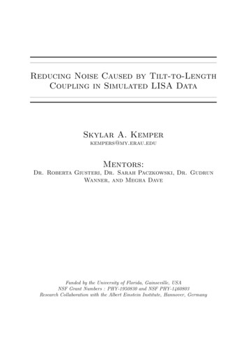
those observed changes include lateral and longitudinal shifts which are depicted by thegreen arrows. Outside of lateral and longitudinal shifts, we also observed changes to themeasurement beams waist size and waist location, see figure (3).Figure 2: Diagram depicting the IfoCAD simulation in terms of what is theoreticallyhappening if the simulation were real light beams and equipment.7

Figure 3: Diagram depicting the changes impacting the measurement beam waist forthe IfoCAD simulation. Where the beam waist itself is defined by W0 , the changes tothe beam waist size are represented by W1 showing the squeezing and expanding of thebeam waist. W2 shows the beam waist location changes, where the beam waist W0 ismoved along the axis, changing the measurement beam divergence and shape.The equation used to determine the TTL estimations is derived through creatinggraphs of the results. To begin, the first graph depicts the relationship between LPSoffset (m) and the angle of the offset (rad). The data is fit to a second order polynomialas depicted by equation (4). Or a first order polynomial as depicted in equation (5).LP S Cm 2φrad2(4)mφrad(5)LP S CmNext, a second graph is created using the Coefficient (C) ( rad2 ) values from the first8

graph and equations (4) - (5). This graph depicts the Longitudinal or Lateral Offset ofmQPD (m) from the Coefficient value ( rad2 ). The second graph is used to find the valuem2for the final Coefficient (Coeff.) ( radm ) using equation (6).Coef f C(1, 1) dlong C(1, 2)(6)rad) represent the displacement longitudinal or lateral from the QPD.Where dlong ( rtHzUsing the values from equation (6), equation (7) can be created to find a TTL estimation.T T L Estimation 2 Coef f φ φof f(7)Where φof f is the offset of the angle (φ) (rad) given in equation (8) for the data beinganalyzed.φof f 50 10 6(8)The final equation used to determine the TTL estimation comes from combiningequations (5) and (6) to create equation (9). The intercept comes from the intercept ofeach line from the secondary graphs (2).T T LEstimation 2 φof f φ Coef f dlong Intercept3.2(9)Tilt-to-Length Subtraction through Time Delay InterferometryThere are two central types of noises which impact LISA, Instrumental noise and GalacticForeground Noise. Galactic Foreground Noise is composed of all the signals LISA will9

measure from the galaxy. A majority of the noise comes from double white dwarf binarieswhich is why a lot of the time other sources are ignored in favor of just the white dwarfbinaries. After a source has been identified, however, it can be subtracted from theoverall Galactic Foreground Noise which allows us to whittle it down to just what canbe resolved. The residual is what composes the the background noise.For this project the Galactic Foreground noise is simulated using a LISAsolve softwarein which every binary is modeled in the frequency domain and only double binary whitedwarfs are simulated. Unresolved Galactic Foreground Noise comes from subtractingresolved binary sources from the simulated population of binaries, creating the noiseused in this project.44.1ResultsGeometric TTL EstimationsThrough running the simulation described under Geometric TTL estimation’s theorysection, without changing any variables, we were able to develop a graph for the angleand the LPS with a rotation at the photodiode center. However, in order to observe theimpacts of longitudinal and lateral QPD shifts we added those shifts on to two separategraphs to observe the changes, see figures (4) and (5) respectively.10